Data Science for Electron Microscopy
Lecture 1: Introduction

Prof. Dr. Philipp Pelz

FAU Erlangen-Nürnberg

Institute of Micro- and Nanostructure Research

Outline

Formalities

Introduction
to
Electron
Microscopy
Data

Basic Pytorch
Knowledge

.

Formalities

Course Website
8-9 lectures
1 graded miniproject (40% of the final grade)
- use of AI tools is allowed:
  - e.g. Github Copilot (free for students)
  - e.g. Cursor (paid)
1 graded exam (60% of the final grade)

Book that covers many topics of the course

Interactive deep learning book with code, math, and discussions
Implemented with PyTorch, NumPy/MXNet, JAX, and TensorFlow
Adopted at 500 universities from 70 countries
We will use the pytorch framework for our coding

STEM capabilities

Imaging (Z–contrast, light-element, phase-contrast)
4D-STEM diffraction & orientation mapping
Spectroscopies (EELS/XEDS, plasmonics)
Tomography down to every atom
Simulation & data-science backbone

STEM operating modes

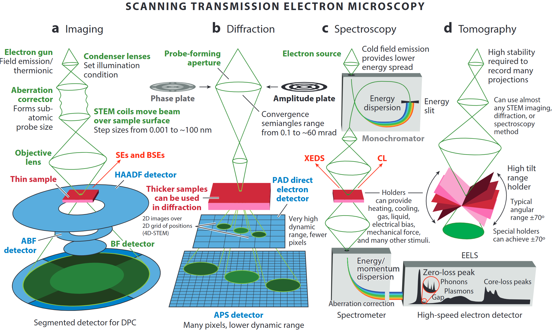
A modern microscope can switch on the fly between
- incoherent imaging,
- diffraction/4D-STEM,
- EELS / XEDS spectroscopy, and
- tilt-series tomography
“A synchrotron in a microscope”: one tool covers Å-to-µm length-scales and meV-to-keV energy-scales.

4DSTEM - Diffraction from a crystalline sample

Ideally, the diffracted signal is simply a 2D Fourier transform of the projected potential, multiplied by the probe intensity.
Thus the position and intensity of Bragg disks of each diffraction pattern acts as a fingerprint for the local structure and orientation of the (crystal) sample.
Interpretation is complicated by multiple / dynamical scattering (thickness effects), overlapping grains, background signals.

4DSTEM - Diffraction from a amorphous sample

Ideally, the diffracted signal is simply a 2D Fourier transform of the projected potential, multiplied by the probe intensity.
The position and shape of amorphous halos of each diffraction pattern acts as a fingerprint for the local structure factor, given by the mean atomic arrangement.
Interpretation is complicated by multiple / dynamical scattering (thickness effects), overlapping grains, more than crystal diffraction.

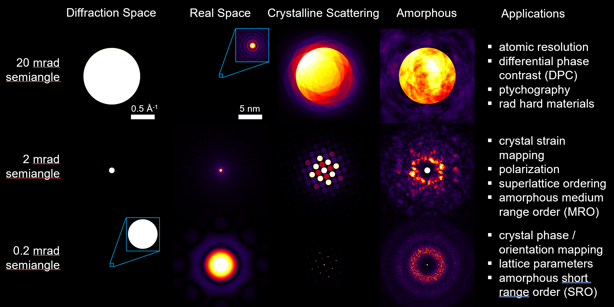
4DSTEM - Design of experiments

Single-atom Z-contrast

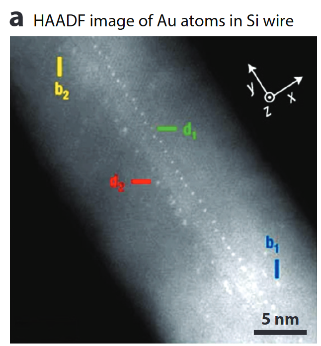
HAADF collects high-angle incoherent scattering → intensity ∝ Z^1.6 – Z^1.9
Detects & counts individual heavy atoms, even inside a nanowire.
Sub-picometre column-position metrology enables strain & segregation studies.

Calibrated composition imaging

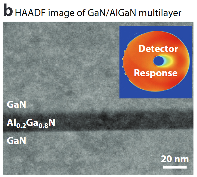
Absolute detector-response calibration converts HAADF signal to atomic areal density .
Enables nm-scale composition profiles (here Al₀.₂Ga₀.₈N) & local thickness determination to ≈1 nm.

Seeing light elements – ABF/BF

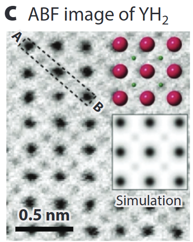
Annular Bright-Field (ABF) records low-angle transmitted beam: simultaneously heavy & very light atoms (H, Li, O) .
Quantitative contrast modelling (multislice + frozen phonon) allows thickness & defocus refinement.

Mapping internal fields – DPC

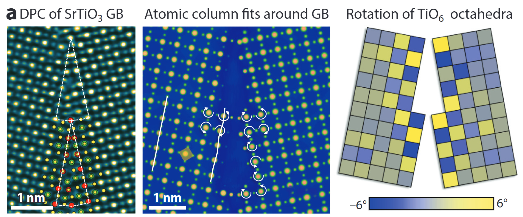
Segmented / pixelated detectors yield differential phase-contrast (DPC) images.
Linear to projected electric-field; with sample flip or advanced analysis → magnetic induction too .
Here: TiO₆ octahedra rotations and GB polarity resolved at the picometre level.

4D-STEM diffraction & orientation mapping

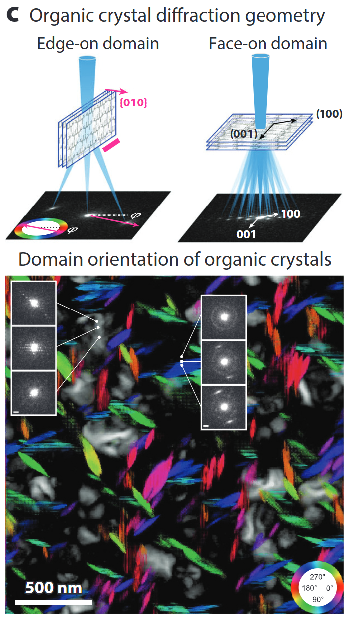
Pixelated cameras record a CBED pattern at every probe position → 4D data cube.
From disks, extract local strain, orientation, thickness, even (via ptychography) phases beyond the probe NA.
Matching experiment to simulation (thermal + inelastic) achieves quantitative thickness/chemistry

Spectroscopy – EELS/XEDS

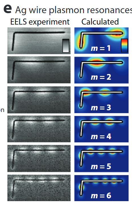
STEM-EELS resolves plasmons (few eV), phonons (meV) & core-loss fine structure (bonding, oxidation).
Combined with modelling (BEM, DFT, multiplet) for nanophotonic mode mapping .
Parallel XEDS gives simultaneous 3-D elemental maps.

Atomic electron tomography

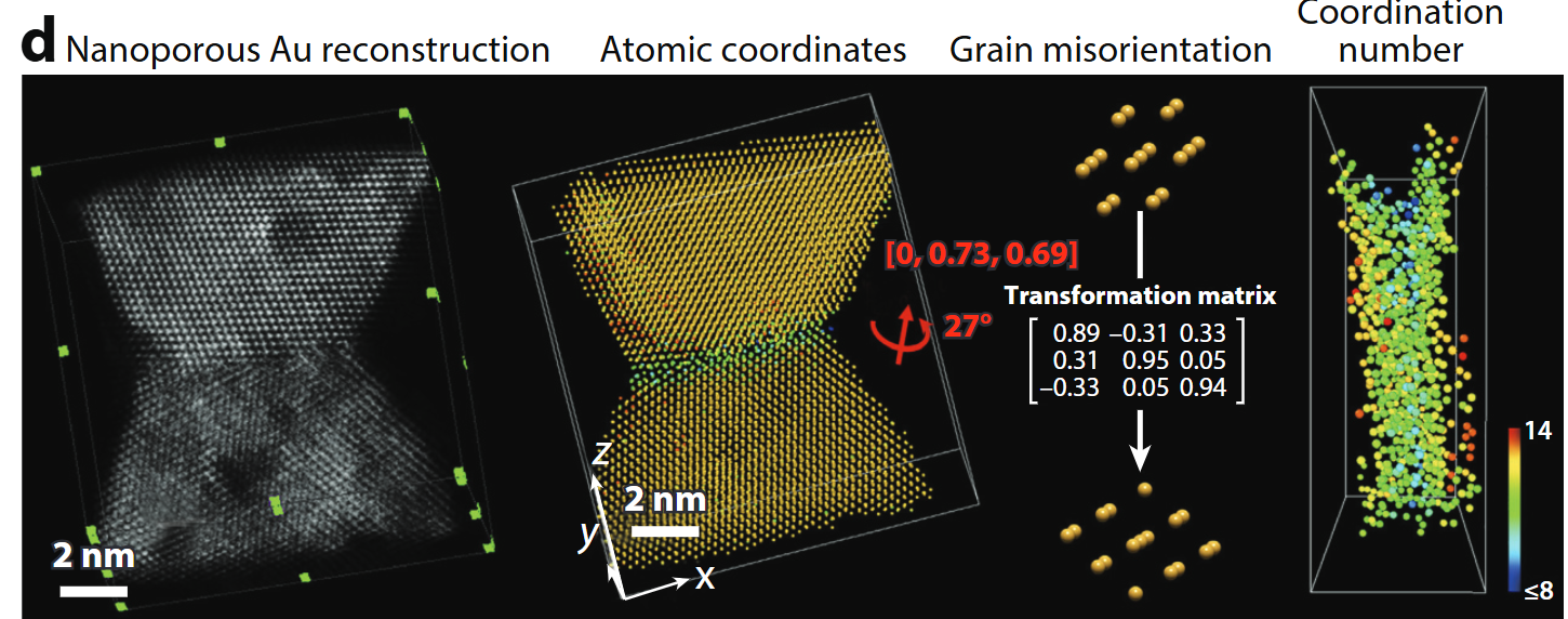
Tilt-series HAADF/ptychography + iterative reconstruction → 3-D coordinates of every atom in ≤20 nm objects .
Enables full strain tensors, defect cores, compositional ordering.

Simulation accelerators – PRISM

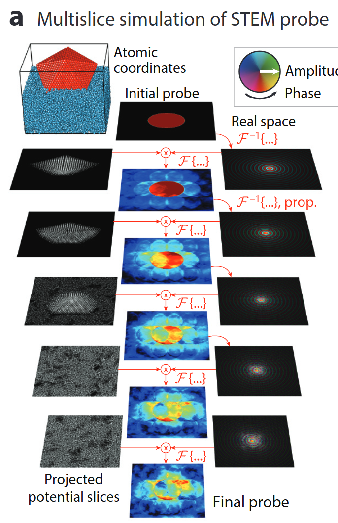
Quantitative STEM hinges on ab-initio accurate multislice simulations.
PRISM re-uses plane-wave slices → orders-of-magnitude faster with <1 % error .
Powers real-time experiment steering & big-data 4D-STEM analysis.

Take-aways

Modern aberration-corrected STEM delivers Å-resolution imaging, diffraction, spectroscopy & tomography within one instrument.
Quantification (composition, fields, 3-D structure) now matches the resolution.
Open-source simulation & Python toolchains are key enablers for truly quantitative materials science.

The data-driven TEM framework (Figure 1)

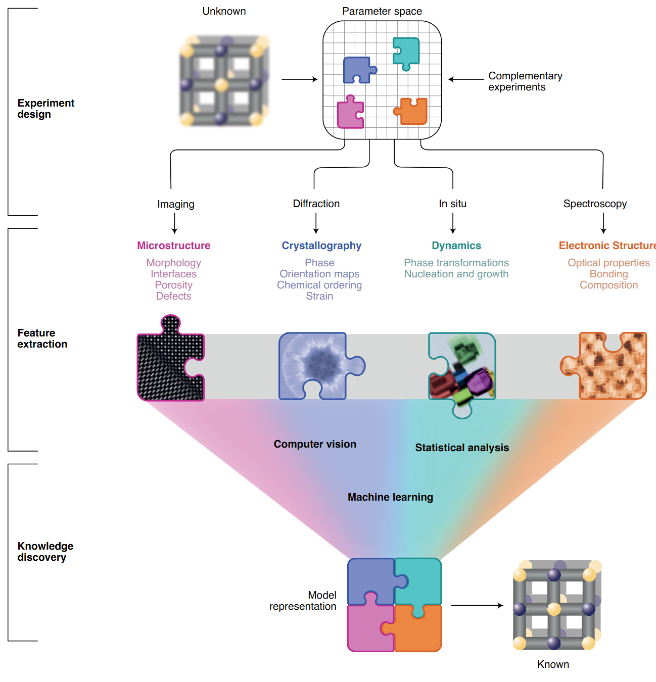
Three nested layers turn unknown samples → quantifiable descriptors
1. Experiment design
2. Feature extraction
3. Knowledge discovery
Open, interoperable control + AI links all layers into a virtuous cycle.

① Experiment design (Fig 1 top)

GPU-accelerated simulations predict detection limits & dose budgets before the first electron hits the sample.
ML mines prior-work databases (future) to recommend optimal imaging / spectroscopy modes in real time.
Outcome: fewer trial-and-error sessions; cost & time savings.

② Feature extraction (Fig 1 middle)

Records complete data streams (e.g. 4D-STEM diffraction cubes) for flexible post-processing
Combines complementary modalities to overcome projection & damage artefacts.
Requires automation and low-level access for batch surveys & in-situ studies.

③ Knowledge discovery (Fig 1 bottom)

AI/ML trained on physical models classifies multidimensional signals → structure, bonding, dynamics.
FAIR data standards and open repositories enable meta-analysis & reproducibility.
Vision: adaptive microscopy where data choose the next experiment step on-the-fly.

Detectors drive the data deluge (Figure 2 a)

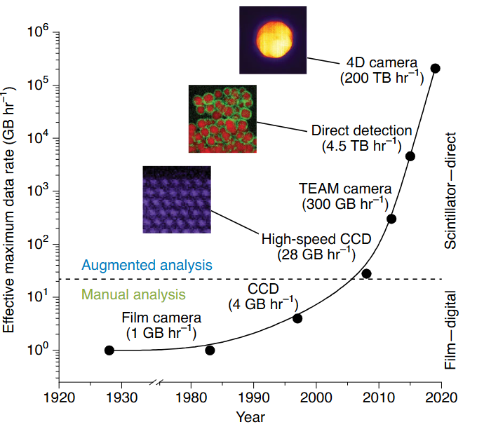
From film (1 GB h⁻¹) to 4D pixelated cameras (200 TB h⁻¹) – a 10⁸× leap in two decades.
Computing & storage must scale in lock-step; edge processing at the microscope becomes essential.

Workflow evolution (Figure 2 b)

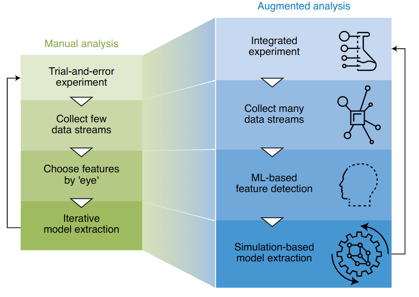
Manual: choose features “by eye”, serial data, iterative models.
Augmented: collect many data streams, ML finds features, simulation-based model extraction.
Integrated experiment control enables closed-loop, crowd-sourced materials discovery.

Take-aways

Modern STEM now spans Å-scale resolution & petabyte-scale data.
A three-layer, open architecture (design → extraction → discovery) lets AI and simulation turn data into insight.
Detector advances + FAIR data infrastructure set the stage for truly adaptive, autonomous microscopy.

Course outline

Intro (13.05.2025)
Regression and Sensor Fusion (20.05.2025)
CNNs (27.05.2025)
Classification, Segmentation, AutoEncoders (03.06.2025)
Miniproject (3.6. - 24.6.2025) concurrent to lectures
Project Presentations, GANs (24.06.2025)
Gaussian Processes Introduction (01.07.2025)
Gaussian Processes Applications (08.07.2025)
Advanced Forward Models for Imaging: Tomography, Diffractive Imaging (15.07.2025)
Repetition (29.07.2025)

Miniproject

In the miniproject, you will test multiple deep neural network architectures on one of four microscopy-related tasks.
You should summarize your results in a short presentation (5 minutes + 2 minutes discussion) and deliver a Jupyter Notebook with your code and results.
The miniproject will be graded and will count as 40% towards your final grade.

Data Manipulation

Data handling requires two main tasks:
- Data acquisition
- Data processing
Key concepts for data manipulation:
- \(n\)-dimensional arrays (tensors) are fundamental
- Modern deep learning frameworks use tensor classes:
  - ndarray in MXNet
  - Tensor in PyTorch and TensorFlow
  - Similar to NumPy’s ndarray with additional features
- Key advantages of tensor classes:
  - Support automatic differentiation
  - GPU acceleration for numerical computation
  - NumPy only runs on CPUs

Getting Started 1

Import PyTorch:

import torch

Tensor basics:
- Vector: tensor with one axis
- Matrix: tensor with two axes
- \(k^\mathrm{th}\) order tensor: tensor with \(k > 2\) axes
Tensor creation:
- Use arange(n) for evenly spaced values (0 to n-1)
- Default storage: main memory
- Default computation: CPU-based

Getting Started 2

x = torch.arange(12, dtype=torch.float32)
x

tensor([ 0.,  1.,  2.,  3.,  4.,  5.,  6.,  7.,  8.,  9., 10., 11.])

Tensor elements:
- Each value is an element
- Use numel() to get total element count
- Use shape attribute to get dimensions

x.numel()
x.shape

torch.Size([12])

Reshaping tensors:
- Use reshape to change shape without changing values
- Example: vector (12,) → matrix (3, 4)
- Elements maintain order (row-major)

X = x.reshape(3, 4)
X

tensor([[ 0.,  1.,  2.,  3.],
        [ 4.,  5.,  6.,  7.],
        [ 8.,  9., 10., 11.]])

Getting Started 3

Shape inference:
- Use -1 to automatically infer one dimension
- Example: x.reshape(-1, 4) or x.reshape(3, -1)
- Given size \(n\) and shape (\(h\), \(w\)), \(w = n/h\)
Common tensor initializations:
- Zeros: torch.zeros((2, 3, 4))
- Ones: torch.ones((2, 3, 4))
- Random (Gaussian): torch.randn(3, 4)
- Custom values: torch.tensor([[2, 1, 4, 3], [1, 2, 3, 4], [4, 3, 2, 1]])

Indexing and Slicing 1

Access methods:
- Indexing (0-based)
- Negative indexing (from end)
- Slicing (start:stop)
- Single index/slice applies to axis 0

X[-1], X[1:3]

(tensor([ 8.,  9., 10., 11.]),
 tensor([[ 4.,  5.,  6.,  7.],
         [ 8.,  9., 10., 11.]]))

Element modification:
- Use indexing for assignment
- Example: X[1, 2] = 17

Indexing and Slicing 2

Multiple element assignment:
- Use indexing on left side of assignment
- : selects all elements along an axis
- Works for vectors and higher-dimensional tensors

X[:2, :] = 12
X

tensor([[12., 12., 12., 12.],
        [12., 12., 12., 12.],
        [ 8.,  9., 10., 11.]])

Operations 1

Elementwise operations:
- Apply scalar operations to each element
- Work with corresponding element pairs
- Support unary operators (e.g., \(e^x\))
- Signature: \(f: \mathbb{R} \rightarrow \mathbb{R}\)

torch.exp(x)

tensor([162754.7969, 162754.7969, 162754.7969, 162754.7969, 162754.7969,
        162754.7969, 162754.7969, 162754.7969,   2980.9580,   8103.0840,
         22026.4648,  59874.1406])

Operations 2

Binary operations:
- Work on pairs of real numbers
- Signature: \(f: \mathbb{R}, \mathbb{R} \rightarrow \mathbb{R}\)
- Common operators:
  - Addition (+)
  - Subtraction (-)
  - Multiplication (*)
  - Division (/)
  - Exponentiation (**)

x = torch.tensor([1.0, 2, 4, 8])
y = torch.tensor([2, 2, 2, 2])
x + y, x - y, x * y, x / y, x ** y

(tensor([ 3.,  4.,  6., 10.]),
 tensor([-1.,  0.,  2.,  6.]),
 tensor([ 2.,  4.,  8., 16.]),
 tensor([0.5000, 1.0000, 2.0000, 4.0000]),
 tensor([ 1.,  4., 16., 64.]))

Operations 3

Tensor concatenation:
- Use torch.cat with list of tensors
- Specify axis for concatenation
- Shape changes:
  - Axis 0: sum of input axis-0 lengths
  - Axis 1: sum of input axis-1 lengths

X = torch.arange(12, dtype=torch.float32).reshape((3,4))
Y = torch.tensor([[2.0, 1, 4, 3], [1, 2, 3, 4], [4, 3, 2, 1]])
torch.cat((X, Y), dim=0), torch.cat((X, Y), dim=1)

(tensor([[ 0.,  1.,  2.,  3.],
         [ 4.,  5.,  6.,  7.],
         [ 8.,  9., 10., 11.],
         [ 2.,  1.,  4.,  3.],
         [ 1.,  2.,  3.,  4.],
         [ 4.,  3.,  2.,  1.]]),
 tensor([[ 0.,  1.,  2.,  3.,  2.,  1.,  4.,  3.],
         [ 4.,  5.,  6.,  7.,  1.,  2.,  3.,  4.],
         [ 8.,  9., 10., 11.,  4.,  3.,  2.,  1.]]))

Operations 4

Logical operations:
- Create binary tensors via logical statements
- Example: X == Y creates tensor of 1s and 0s
- Sum operation: X.sum() reduces to single element

X == Y
X.sum()

tensor(66.)

Broadcasting

Mechanism for elementwise operations with different shapes:
- Step 1: Expand arrays along length-1 axes
- Step 2: Perform elementwise operation

a = torch.arange(3).reshape((3, 1))
b = torch.arange(2).reshape((1, 2))
a + b

tensor([[0, 1],
        [1, 2],
        [2, 3]])

Saving Memory 1

Memory allocation issues:
- Operations create new memory allocations
- Example: Y = X + Y creates new memory
- Check with id() function
- Undesirable for:
  - Frequent parameter updates
  - Multiple variable references

Saving Memory 2

In-place operations:
- Use slice notation: Y[:] = <expression>
- Use zeros_like for initialization
- Use X[:] = X + Y or X += Y for efficiency

Z = torch.zeros_like(Y)
Z[:] = X + Y
X += Y

Conversion to Other Python Objects

NumPy conversion:
- X.numpy(): Tensor → NumPy array
- torch.from_numpy(A): NumPy array → Tensor
- Shared memory between conversions
Scalar conversion:
- Use item() or built-in functions
- Example: float(a), int(a)

Summary

Tensor class features:
- Data storage and manipulation
- Construction routines
- Indexing and slicing
- Basic mathematics
- Broadcasting
- Memory-efficient operations
- Python object conversion

Exercises

Experiment with different conditional statements:
- Try X < Y and X > Y
- Observe resulting tensor types
Test broadcasting with 3D tensors:
- Try different shapes
- Verify results match expectations

Automatic Differentiation

Key points about derivatives in deep learning:
- Essential for optimization algorithms
- Used in training deep networks
- Manual calculation is:
  - Tedious
  - Error-prone
  - More difficult with complex models
Modern deep learning frameworks provide:
- Automatic differentiation (autograd)
- Computational graph tracking
- Backpropagation implementation
  - Works backwards through graph
  - Applies chain rule
  - Efficient gradient computation

import torch

A Simple Function

Goal: Differentiate \(y = 2\mathbf{x}^{\top}\mathbf{x}\) with respect to \(\mathbf{x}\)
Initial setup:

x = torch.arange(4.0)
x

tensor([0., 1., 2., 3.])

Gradient storage considerations:
- Need space to store gradients
- Avoid new memory allocation for each derivative
- Important because:
  - Deep learning requires many derivative computations
  - Same parameters used repeatedly
  - Memory efficiency crucial
- Gradient shape matches input vector shape

x.requires_grad_(True)
x.grad  # The gradient is None by default

Function calculation:

y = 2 * torch.dot(x, x)
y

tensor(28., grad_fn=<MulBackward0>)

Gradient computation:
- Use backward() method
- Access via grad attribute
- Expected result: \(4\mathbf{x}\)

y.backward()
x.grad
x.grad == 4 * x

tensor([True, True, True, True])

Important note about gradient accumulation:
- PyTorch adds new gradients to existing ones
- Useful for optimizing sum of multiple objectives
- Reset with x.grad.zero_()

x.grad.zero_()  # Reset the gradient
y = x.sum()
y.backward()
x.grad

tensor([1., 1., 1., 1.])

Backward for Non-Scalar Variables

Vector derivatives:
- Natural interpretation: Jacobian matrix
- Contains partial derivatives of each component
- Higher-order tensors for higher-order inputs
Common use case:
- Sum gradients of each component
- Often needed for batch processing
- Results in vector matching input shape
PyTorch implementation:
- Requires explicit reduction to scalar
- Uses vector \(\mathbf{v}\) for computation
- Computes \(\mathbf{v}^\top \partial_{\mathbf{x}} \mathbf{y}\)
- Argument named gradient for historical reasons

x.grad.zero_()
y = x * x
y.backward(gradient=torch.ones(len(y)))  # Faster: y.sum().backward()
x.grad

tensor([0., 2., 4., 6.])

Detaching Computation

Purpose: Move calculations outside computational graph
Use cases:
- Create auxiliary terms without gradients
- Focus on direct influence of variables
- Control gradient flow
Example scenario:
- z = x * y and y = x * x
- Want direct influence of x on z
- Solution: Detach y to create u
- Results in:
  - Same value as y
  - No gradient flow through u
  - Direct computation of z = x * u

x.grad.zero_()
y = x * x
u = y.detach()
z = u * x

z.sum().backward()
x.grad == u

tensor([True, True, True, True])

Important notes:
- Detaches ancestors from graph
- Original graph for y persists
- Can still compute gradients for y

x.grad.zero_()
y.sum().backward()
x.grad == 2 * x

tensor([True, True, True, True])

Gradients and Python Control Flow

Key feature: Works with dynamic computation paths
Supports:
- Conditional statements
- Loops
- Arbitrary function calls
- Variable-dependent control flow
Example function:

def f(a):
    b = a * 2
    while b.norm() < 1000:
        b = b * 2
    if b.sum() > 0:
        c = b
    else:
        c = 100 * b
    return c

Implementation details:
- Graph built during execution
- Specific path for each input
- Supports backward pass after execution
- Works with linear functions and piecewise definitions

a = torch.randn(size=(), requires_grad=True)
d = f(a)
d.backward()
a.grad == d / a

tensor(True)

Real-world applications:
- Text processing with variable lengths
- Dynamic model architectures
- Statistical modeling
- Impossible to compute gradients a priori

Discussion

Impact of automatic differentiation:
- Massive productivity boost
- Enables complex model design
- Frees practitioners for higher-level tasks
Technical aspects:
- Optimization of autograd libraries
- Compiler and graph manipulation tools
- Memory efficiency
- Computational efficiency
Basic workflow:
1. Attach gradients to target variables
2. Record target value computation
3. Execute backpropagation
4. Access resulting gradient

Exercises

Backpropagation behavior:
- Run function twice
- Observe and explain results
Control flow analysis:
- Change a to vector/matrix
- Analyze non-scalar results
- Explain computation changes
Automatic differentiation practice:
- Plot \(f(x) = \sin(x)\)
- Plot derivative using autograd
- Avoid using known derivative formula

Chain rule exercise:
- Function: \(f(x) = ((\log x^2) \cdot \sin x) + x^{-1}\)
- Create dependency graph
- Compute derivative using chain rule
- Map terms to dependency graph
Let \(f(x) = ((\log x^2) \cdot \sin x) + x^{-1}\). Write out a dependency graph tracing results from \(x\) to \(f(x)\).

Use the chain rule to compute the derivative \(\frac{df}{dx}\) of the aforementioned function, placing each term on the dependency graph that you constructed previously.

References

Ophus, Colin. 2023. “Quantitative Scanning Transmission Electron Microscopy for Materials Science: Imaging, Diffraction, Spectroscopy, and Tomography.” Annual Review of Materials Research 53 (1): 105–41.

Spurgeon, Steven R., Colin Ophus, Lewys Jones, Amanda Petford-Long, Sergei V. Kalinin, Matthew J. Olszta, Rafal E. Dunin-Borkowski, et al. 2020. “Towards Data-Driven Next-Generation Transmission Electron Microscopy.” Nature Materials, October, 1–6. https://doi.org/10/ghhtjq.

Data Science for Electron Microscopy Lecture 1: Introduction

Outline

Formalities

Introduction to Electron Microscopy Data

Basic Pytorch Knowledge

.

Formalities

Book that covers many topics of the course

STEM capabilities

STEM operating modes

4DSTEM - Diffraction from a crystalline sample

4DSTEM - Diffraction from a amorphous sample

4DSTEM - Design of experiments

Single-atom Z-contrast

Calibrated composition imaging

Seeing light elements – ABF/BF

Mapping internal fields – DPC

4D-STEM diffraction & orientation mapping

Spectroscopy – EELS/XEDS

Atomic electron tomography

Simulation accelerators – PRISM

Take-aways

The data-driven TEM framework (Figure 1)

① Experiment design (Fig 1 top)

② Feature extraction (Fig 1 middle)

③ Knowledge discovery (Fig 1 bottom)

Detectors drive the data deluge (Figure 2 a)

Workflow evolution (Figure 2 b)

Take-aways

Course outline

Miniproject

Data Manipulation

Getting Started 1

Getting Started 2

Getting Started 3

Indexing and Slicing 1

Indexing and Slicing 2

Operations 1

Operations 2

Operations 3

Operations 4

Broadcasting

Saving Memory 1

Saving Memory 2

Conversion to Other Python Objects

Summary

Exercises

Automatic Differentiation

A Simple Function

Backward for Non-Scalar Variables

Detaching Computation

Gradients and Python Control Flow

Discussion

Exercises

References

Data Science for Electron Microscopy
Lecture 1: Introduction

Introduction
to
Electron
Microscopy
Data

Basic Pytorch
Knowledge