Data Science for Electron Microscopy
Week 3: Linear algebra, PCA & spectral unmixing

Prof. Dr. Philipp Pelz

FAU Erlangen-Nürnberg

Institute of Micro- and Nanostructure Research

Recap: where we left off

• Week 2: EM data formation. Specimen → interaction → detector → digitisation → metadata. Every stage leaves a fingerprint on the numbers.
• Noise model → likelihood → loss: Gaussian noise gives MSE, Poisson counts give the Poisson NLL, mixed noise calls for a variance-stabilising transform (Anscombe).
• Every EM pixel is a count, so the variance depends on the signal. Low-dose data are noisy no matter what you do afterwards.
• Gap: a spectrum image holds 10⁴–10⁵ spectra with hundreds of channels each. We need a compact representation that is also physically interpretable.
• Today: the linear algebra behind that representation. First PCA, which finds the subspace. Then NMF / MCR, which turn the subspace into phases.

• Open by asking: who completed the Week 2 notebook? The low-count fit should have shown that the shortcut losses (count-weighted χ², Anscombe + MSE) are biased and that plain MSE wastes dose compared with the Poisson NLL. Keep that result in mind, because today it comes back as “weight before PCA”.
• The one point to land: Week 2 said that the noise model decides the loss. Today the same principle decides the decomposition. Plain PCA is least squares, i.e. it implicitly assumes Gaussian noise. Poisson data need weighting, or a Poisson-divergence NMF.
• Misconception to preempt: “I did not enjoy linear algebra in my physics degree.” This week’s linear algebra is geometric and intuition-first: projections, ellipses, triangles. If you can picture a stretched ellipse and a triangle of mixtures, you already have the core idea.
• EM anchor: an EELS spectrum image is a 3-D tensor (x, y, E), e.g. 128 × 128 pixels × 1024 channels, which is about 16 million numbers. The chemistry lives in maybe 3–5 of them per pixel.
• Pacing note: the first half (geometry, SVD, PCA, scree, denoising, ~45 min) is familiar ground and should move briskly. Protect ~30 min for the new second half: EELS preprocessing, NMF, MCR-ALS and unmixing pitfalls.
• Transition: “Two questions anchor today.”

Today’s question

• Why does PCA denoise an EELS spectrum image? Because the signal lives in a low-dimensional subspace, while the noise spreads across all directions.
• Why are PCA components not phases, and what gives us phases? Non-negativity and mixing constraints: NMF, MCR-ALS, endmember unmixing.
• Road map: geometry & projection · SVD & PCA · scree & denoising · EELS preprocessing & Poisson weighting · linear mixing, NMF & MCR-ALS · unmixing pitfalls · ill-conditioning & limits.
• Self-study: notebooks/week03_pca_nmf_eels.ipynb. Build a 3-phase spectrum image, then compare PCA and NMF against the ground truth.

• Name the payoff upfront. By the end, students can (1) run and read a PCA scree plot, (2) explain why PCA components are signed and not phases, (3) run NMF and state why its answer is not unique, and (4) describe the EELS preprocessing steps that must come before any decomposition.
• The one point to land: PCA answers “how many things vary?”, and unmixing answers “what are the things?”. Both are matrix factorisations X ≈ T·S; they differ only in the constraints.
• Misconception to preempt: “NMF replaces PCA.” No. In practice PCA is used first (denoise, choose K) and NMF/MCR second (interpret). Both run in the same pipeline.
• Forward link: Week 4 uses least squares = projection (today’s geometry) for regression. Week 9 generalises PCA to non-linear autoencoders, and constrained autoencoders generalise NMF.
• Transition: “Here is what you should be able to do at the end.”

Learning outcomes

By the end of this week you can:

1. Reshape a spectrum image into a data matrix \(\mathbf{X}\in\mathbb{R}^{N\times D}\) (rows = pixels) and back.
2. Explain SVD geometrically and connect singular values to the variance per principal component.
3. Choose the number of components \(K\) from a scree plot, and name the ways that choice can go wrong.
4. Describe the EELS preprocessing chain: energy alignment → power-law background → normalisation → Poisson weighting.
5. Formulate NMF and MCR-ALS as constrained factorisations, and explain multiplicative updates and alternating least squares.
6. Diagnose rotational ambiguity, PCA truncation bias and rare-phase loss, using residual maps and restarts.

• These outcomes map directly to exam must-know statements (see the must-know slide at the end). Outcomes 4–6 are new this year. They are the practical skills a microscopist needs before trusting any “phase map” produced by software such as HyperSpy.
• The one point to land: outcome 6 is the most important one. Every factorisation produces a picture, and the craft is knowing when the picture is lying.
• Pacing note: do not read the list out loud. Point at 4–6 and say “this is what is new compared to a generic ML course”.
• Timing plan (90 min, lecture path ≈ 85 min incl. ~5 min slack for questions):
  • 0–5 min: recap, today’s question, learning outcomes.
  • 5–17 min: vectors & projection, data matrix & reshape, projection onto a subspace, least squares = projection.
  • 17–29 min: SVD (rotate–stretch–rotate, factors), Eckart–Young, PCA as max variance, PCA in NumPy.
  • 29–40 min: scree plot, choosing K, PCA denoising with k components, why it works, eigen-spectra & score maps.
  • 40–48 min: EELS preprocessing chain, power-law background & alignment, Poisson weighting.
  • 48–65 min: linear mixing model, known endmembers & simplex, NMF, multiplicative updates, PCA vs NMF, MCR-ALS.
  • 65–73 min: pitfall 1 (rotational ambiguity), pitfall 2 (truncation bias), decision table.
  • 73–78 min: ill-conditioning (κ), limits of linear methods.
  • 78–85 min: summary, must-know takeaways, Week 4 teaser, self-study/notebook.
  • 85–90 min: slack for questions.
• Backup slides after “Continue” (Potapov weighting paper, deep-mantle NMF case study, covariance matrix, matrices as transformations, ill-conditioning in EM + diagnostic) are for questions only.
• Transition: “Start with the simplest thing: what is a vector?”

Vectors, dot products and projection

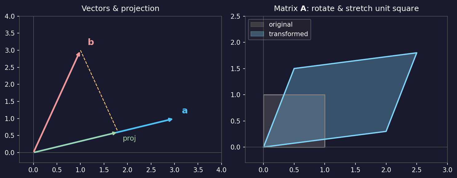
Projection of \(\mathbf{b}\) onto the direction of \(\mathbf{a}\); the residual (orange dashed) is orthogonal.

• One EELS spectrum with \(D\) channels is a vector \(\mathbf{x}\in\mathbb{R}^D\), a point in \(D\)-dimensional space.
• Dot product \(\mathbf{a}^T\mathbf{b}=\|\mathbf{a}\|\|\mathbf{b}\|\cos\theta\) measures alignment; \(=0\) ⟹ orthogonal.
• Projection onto a unit vector \(\hat{\mathbf{a}}\): \(c=\hat{\mathbf{a}}^T\mathbf{b}\), \(\ \text{proj}_{\mathbf{a}}\mathbf{b}=c\,\hat{\mathbf{a}}\).
• The residual \(\mathbf{b}-c\,\hat{\mathbf{a}}\) is ⊥ \(\mathbf{a}\). “How much lies along \(\mathbf{a}\)?” is what PCA asks in every direction.

• Draw two arrows on the board. Ask: what does it mean for two spectra to be “similar”? Answer: their dot product is large (they point in almost the same direction). Two chemically distinct spectra (oxide vs metal) are nearly orthogonal. Norm \(\|\mathbf{a}\|=\sqrt{\mathbf{a}^T\mathbf{a}}\) is the length of the arrow.
• Work through the picture: blue arrow \(\mathbf{a}\), red arrow \(\mathbf{b}\), green arrow the projection, orange dashed the residual meeting \(\mathbf{a}\) at a right angle.
• The one point to land: projection = the “shadow” of \(\mathbf{b}\) on the line of \(\mathbf{a}\) = the closest point on that line. The scalar \(c\) tells you how much of \(\mathbf{b}\) is “explained” by the direction \(\mathbf{a}\).
• Misconception to preempt: “a vector is just a list of numbers.” It is, but it also has a geometric meaning (direction + magnitude) that becomes crucial when we ask “which direction captures the most variance?”
• EM anchor: projecting an EELS spectrum onto a unit-normalised reference Fe-L edge spectrum gives a “match score”, i.e. how much Fe-L edge is in the spectrum. This is reference fitting / spectral unmixing in one formula.
• Forward link: least-squares regression (Week 4) generalises this to projecting onto a subspace spanned by several feature vectors.
• Transition: “Now stack many spectra: the data matrix.”

The data matrix: EM spectra as points in high-D space

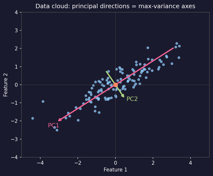
Data cloud with principal directions (arrows): PC1 = direction of maximum spread, PC2 = orthogonal residual.

• Data matrix \(\mathbf{X}\in\mathbb{R}^{N\times D}\): one row per pixel spectrum, one column per energy channel (this week’s convention).
• Each spectrum is a point in \(\mathbb{R}^{1024}\); the cloud occupies only a tiny corner of that space.
• \(K\) distinct phases ⟹ the spectra lie (approximately) on a \(K\)-dimensional subspace. Two phases → a 2-D plane in \(\mathbb{R}^{1024}\).
• PCA finds and extracts that subspace.

• A matrix \(\mathbf{A}\) maps vectors, \(\mathbf{y}=\mathbf{Ax}\): it rotates, stretches (and shears) space. Keep that picture for SVD. (Backup slide “Matrices as geometric transformations” if needed.)
• Work through the figure. The points are spectra; the two arrows are the first two principal components. PC1 points along the direction where spectra vary most (chemical difference between phases); PC2 along the second-largest variation.
• The one point to land: a 1024-channel EELS dataset from a two-phase sample is effectively 2-dimensional. Two numbers per spectrum (scores on PC1 and PC2) characterise it; the other 1022 dimensions are noise.
• Misconception to preempt (1): “the data matrix has \(D\) rows (features) and \(N\) columns.” Fields differ. In this course observations (spectra, pixels) are rows, features (channels) are columns. Always check .shape.
• Misconception to preempt (2): “more channels = more information.” More channels can mean more noise in dimensions that carry no signal.
• EM anchor: in a steel sample with austenite and martensite phases, the EELS spectra are nearly constant within each phase; the data cloud is very thin, and K=2 components capture essentially all the signal.
• Forward link: intrinsic dimensionality reappears in Week 9 (autoencoders), where non-linear methods find curved, not flat, low-dimensional structures.
• Transition: “The practical step: how do we get from a datacube to this matrix?”

Reshaping EM data into a matrix: the practical step

ny, nx, ne = eels_map.shape              # (64, 64, 1024) spectrum image
X = eels_map.reshape(ny * nx, ne)        # (4096, 1024): rows = pixels, cols = channels
# ... PCA / NMF on X gives per-pixel scores of shape (4096, K) ...
score_maps = scores.reshape(ny, nx, K)   # back to K images

• Data layout rule: observations (pixels, spectra) in rows; features (channels) in columns.
• Always check X.shape before any analysis — a transposed matrix gives meaningless PCA.

• Walk through it line by line. The reshape from (64, 64, 1024) to (4096, 1024) is the single operation that unlocks PCA (and NMF) for any spectral image. The notebook does exactly this before calling np.linalg.svd.
• The one point to land: the reshape does not change the data — it re-indexes it. Row 0 of X is the spectrum at pixel (0, 0), row 1 the spectrum at pixel (0, 1), and so on. No information is lost.
• Misconception to preempt: “I should reshape as (1024, 4096) because features go in rows.” In NumPy/sklearn observations are always rows. Transposing before PCA finds directions of variance across pixels instead of across channels — a completely different (and wrong) result.
• EM anchor: HyperSpy’s s.decomposition() does this reshape internally. Understanding it means you can use s.get_decomposition_factors() and s.get_decomposition_loadings() with confidence.
• Transition: “Now the core projection geometry.”

Projection onto a subspace

• Approximate a spectrum \(\mathbf{x}\) with \(K\) orthonormal basis vectors (\(\mathbf{v}_i^T\mathbf{v}_j=\delta_{ij}\)). The best approximation is the orthogonal projection: \[\hat{\mathbf{x}} = \sum_{k=1}^{K} (\mathbf{v}_k^T \mathbf{x})\, \mathbf{v}_k = \mathbf{V}_K \mathbf{V}_K^T \mathbf{x}.\]
• Scores \(c_k = \mathbf{v}_k^T \mathbf{x}\): one dot product each, no matrix inversion (orthonormality makes it trivial).
• Residual \(\mathbf{x} - \hat{\mathbf{x}}\) is ⊥ every \(\mathbf{v}_k\). If the basis captures the signal, the residual is noise.
• PCA’s eigenspectra form such a basis, so the scores of different PCs are uncorrelated.

• This is the conceptual heart of both PCA and linear regression. Projecting onto \(K\) orthonormal vectors is just the single-vector projection done \(K\) times and added up.
• The one point to land: “best approximation in the least-squares sense = orthogonal projection.” This is a theorem (the projection theorem), not a convention.
• Computational point: with an orthonormal basis, projecting a new spectrum costs K dot products, O(KD). No system solve.
• Misconception to preempt (1): “I need to choose the basis vectors before projecting.” For a given subspace, yes. PCA finds the optimal basis from the data, then applies this formula.
• Misconception to preempt (2): “orthogonal components are physically independent.” PCA scores are decorrelated in this dataset. If Fe and Cr both track thickness, the PCs encode linear combinations of them, and getting back to element maps needs an extra unmixing step (second half of today).
• EM anchor: projecting onto a reference Fe-L eigenspectrum gives a score \(c_1\) that tracks the Fe content at that pixel. The score map is a chemical map.
• Forward link: orthonormality is also why the Eckart–Young error is just the sum of discarded \(\sigma_k^2\), with no cross-terms.
• Transition: “The same geometry gives least squares with no calculus.”

Least squares = projection (no calculus required)

• Problem: find weights \(\mathbf{w}\) such that \(\mathbf{Xw} \approx \mathbf{y}\) (predict target \(\mathbf{y}\) from features \(\mathbf{X}\)).
• Geometric view: \(\mathbf{Xw}\) can only reach the column space of \(\mathbf{X}\).
• The best approximation is the orthogonal projection of \(\mathbf{y}\) onto that column space.
• Orthogonality condition: the residual \(\mathbf{r} = \mathbf{y} - \mathbf{Xw}\) must be perpendicular to every column of \(\mathbf{X}\), i.e. \(\mathbf{X}^T \mathbf{r} = \mathbf{0}\).
• Substituting: \(\mathbf{X}^T(\mathbf{y} - \mathbf{Xw}) = \mathbf{0}\) → Normal equations: \(\mathbf{X}^T\mathbf{X}\,\hat{\mathbf{w}} = \mathbf{X}^T \mathbf{y}\) Bishop, Christopher M., (2006).

• Draw the classic picture on the board: \(\mathbf{y}\) is an arrow in \(\mathbb{R}^N\) outside the column space (a plane). The projection \(\hat{\mathbf{y}} = \mathbf{X}\hat{\mathbf{w}}\) is the closest point in the plane; the residual drops perpendicularly to the plane.
• The one point to land: “Normal equations” uses “normal” in the sense of perpendicular, not in the sense of Gaussian. The residual must be perpendicular to the feature subspace — that single geometric requirement gives the entire formula, no derivatives needed.
• Misconception to preempt: “I need to know calculus to understand least squares.” The geometric derivation is completely calculus-free. The calculus derivation agrees, which is reassuring — but you do not need it to understand what is happening.
• EM anchor: fitting an EELS background (power-law or polynomial) is a least-squares problem: find the coefficients of the background model that minimise the squared residual in the pre-edge region. The feature matrix \(\mathbf{X}\) is constructed from the background functional form evaluated at each energy channel.
• Forward link: in Week 4 we will compute \(\hat{\mathbf{w}}\) numerically using gradient descent — but understanding the geometric answer (projection) tells us what gradient descent is converging to.
• Transition: “Now for the big tool: Singular Value Decomposition. We will build it as a geometric story.”

SVD: the rotate–stretch–rotate decomposition

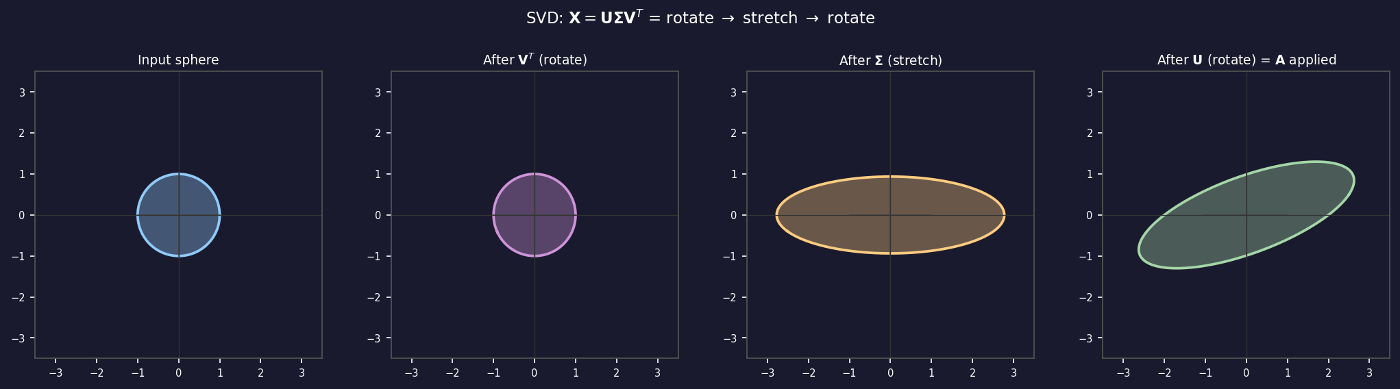
SVD applied to a unit circle: (1) rotate by \(\mathbf{V}^T\), (2) stretch by \(\mathbf{\Sigma}\), (3) rotate by \(\mathbf{U}\) — the result is an ellipse.

• Any matrix: \(\mathbf{X} = \mathbf{U} \boldsymbol{\Sigma} \mathbf{V}^T\) = rotate, stretch, rotate.
• \(\mathbf{V}\) (\(D\times D\)): columns are eigenspectra, directions in channel space.
• \(\boldsymbol{\Sigma}\): singular values \(\sigma_1\ge\sigma_2\ge\ldots\ge0\), the importance of each direction.
• \(\mathbf{U}\) (\(N\times N\)): how strongly each direction is expressed per pixel → score maps.
• \(\mathbf{X} = \sum_k \sigma_k \, \mathbf{u}_k \mathbf{v}_k^T\): a sum of rank-1 “spectral images”.

• Walk through the panels: unit circle (all unit-length inputs) → \(\mathbf{V}^T\) rotates → \(\boldsymbol{\Sigma}\) stretches along the axes into an ellipse → \(\mathbf{U}\) rotates the ellipse.
• The one point to land: the singular values are the semi-axes of the output ellipse. Large \(\sigma\) = strongly stretched direction = lots of information; small \(\sigma\) = likely noise. Each rank-1 term \(\sigma_k\mathbf{u}_k\mathbf{v}_k^T\) is one “spectral variation mode”: the first few describe the chemistry, later ones look like random patterns in both map and spectrum.
• Misconception to preempt (1): “SVD is just eigendecomposition.” SVD works on any (rectangular) matrix. The link: the right singular vectors of the centered data matrix are the eigenvectors of the covariance matrix \(\tilde{\mathbf{X}}^T\tilde{\mathbf{X}}/(N-1)\) (backup slide “The covariance matrix”).
• Misconception to preempt (2): “the first singular vector is the mean spectrum.” Only if you forget to center. PCA subtracts the mean first; PC1 then captures the largest variation around the mean.
• EM anchor: Trebbia and Bonnet (1990) Trebbia, Patrick et al., (1990) introduced SVD/PCA analysis to EELS: the first few singular vectors are real chemical variations, the rest look like noise. This is now standard in HyperSpy.
• Transition: “What happens if we keep only the top few terms of this sum?”

SVD and low-rank approximation (Eckart–Young)

• Truncated SVD: keep only the top \(k\) singular values; set the rest to zero.
• Result: \(\hat{\mathbf{X}}_k = \mathbf{U}_k \boldsymbol{\Sigma}_k \mathbf{V}_k^T\), where subscript \(k\) means “first \(k\) columns.”
• Optimality (Eckart–Young theorem): \(\hat{\mathbf{X}}_k\) is the best rank-\(k\) approximation of \(\mathbf{X}\) in the sense of minimising the Frobenius norm of the reconstruction error: \[\| \mathbf{X} - \hat{\mathbf{X}}_k \|_F = \sqrt{\sigma_{k+1}^2 + \sigma_{k+2}^2 + \cdots}.\]
• Denoising: if signal lives in rank-\(k\) and noise spreads over all ranks, truncation removes noise.
• In Python: U, s, Vt = np.linalg.svd(X, full_matrices=False) — then zero out s[k:].

• The Eckart–Young theorem is the one “theorem” worth naming here — it is the mathematical guarantee that makes PCA trustworthy for denoising. You do not need to prove it, but students should know it exists.
• The one point to land: the reconstruction error from truncating at rank \(k\) is exactly computable from the discarded singular values. This is not an approximation — it is an exact formula. You can always compute how much information you throw away.
• Misconception to preempt: “truncating at rank \(k\) removes only noise.” It removes the directions with smallest singular values, which are dominated by noise if the signal is truly low-rank. But if a rare phase occupies only 1% of pixels, its singular value may be small — and truncation may discard it. Always check the residual.
• EM anchor: a synthetic EELS spectrum image constructed from two latent components plus Poisson noise has true rank 2. Its data matrix will have two large singular values (signal) and many small ones (noise floor). The exact reconstruction error from keeping only rank 2 is \(\sqrt{\sum_{k>2} \sigma_k^2}\).
• Forward link: the scree plot is a visual display of the singular values. The elbow (where the curve transitions from steeply decreasing to flat) marks the boundary between signal and noise.
• Transition: “Now PCA — putting the geometric pieces together.”

PCA: directions of maximum variance

• PCA finds orthonormal directions that maximise the variance of the projected data: PC1 maximises \(\text{Var}(\tilde{\mathbf{X}}\mathbf{v})\) s.t. \(\|\mathbf{v}\|=1\); PC2 ⊥ PC1, and so on.
• PCA = SVD of the centered data: \(\tilde{\mathbf{X}} = \mathbf{X}-\bar{\mathbf{x}} = \mathbf{U}\boldsymbol{\Sigma}\mathbf{V}^T\).
• Loadings (eigenspectra): rows of \(\mathbf{V}^T\). Scores: \(\mathbf{U}\boldsymbol{\Sigma} = \tilde{\mathbf{X}}\mathbf{V}\) → reshape to score maps.
• Equivalently: the eigenvectors of the covariance \(\mathbf{S}=\tilde{\mathbf{X}}^T\tilde{\mathbf{X}}/(N-1)\), i.e. the axes of the data ellipsoid. Variance along PC \(k\): \(\lambda_k = \sigma_k^2/(N-1)\).

• Connect back to the data-cloud figure. The long axis of the ellipse is PC1 (maximum spread), the short axis PC2. SVD finds all of them at once.
• The one point to land: “PCA = SVD of the centered data matrix.” Without centering, the first singular vector just points toward the mean spectrum.
• Scores = “where is each PC strong?” (chemical map). Loadings = “what does each PC look like spectrally?” Together they give the complete interpretation.
• Misconception to preempt (1): “PCA always finds the physically meaningful directions.” Maximum variance may be an instrumental artefact (thickness, beam drift). In EELS of two-phase steel, PC1 often captures thickness and PC2 the chemical contrast.
• Misconception to preempt (2): “the covariance matrix is N × N.” It is D × D (1024 × 1024 for EELS), which is why PCA is feasible for huge pixel counts — and SVD gives its eigenvectors without ever forming it.
• Naming trap: HyperSpy calls the score maps “loadings” and the eigenspectra “factors”. Always check shapes.
• Transition: “In code, all of this is five lines.”

PCA in five lines of NumPy

import numpy as np

# ✅ CORRECT full pipeline — copy this version
mean_spectrum = X.mean(axis=0)                                 # (D,) mean of original data
X_centered    = X - mean_spectrum                              # center before SVD
U, s, Vt      = np.linalg.svd(X_centered, full_matrices=False) # core computation
K = 3                                                          # chosen from scree plot

# Scores (chemical maps): how strongly each PC is expressed per pixel
scores       = X_centered @ Vt[:K].T        # shape (N, K)

# Eigenspectra (spectral shapes): rows of Vt[:K], shape (K, D)
eigenspectra = Vt[:K]                       # already unit-norm and orthogonal

# Reconstruct (denoise): restore mean to get back to original scale
X_denoised   = scores @ eigenspectra + mean_spectrum  # shape (N, D)

• Walk through each line carefully. Students who did the Week 1 notebook will recognise the array operations. The only new call is np.linalg.svd.
• The one point to land: the entire PCA pipeline — center, SVD, choose K, reconstruct — is five lines of NumPy. Every line corresponds to a geometric operation from the slides. There is no black box.
• Misconception to preempt: “I forgot to add the mean back in the reconstruction.” This is the most common error. The SVD was computed on the centered data; the reconstruction is in centered space. To get back to the original scale, you must add the mean spectrum to every reconstructed row. Forgetting this gives systematically wrong intensities.
• Common mistake students make: writing X_denoised = scores @ eigenspectra + X_centered.mean(axis=0) — this uses the mean of the already-centered data (which is ≈ zero), so the mean is NOT restored and every reconstructed spectrum will have systematically wrong absolute intensities. Always save mean_spectrum = X.mean(axis=0) from the original un-centered data before centering.
• EM anchor: hyperspy does this automatically — s.decomposition() stores the mean internally and adds it back in s.get_decomposition_model(). Understanding why this step exists means you can implement it outside hyperspy.
• Forward link: the notebook in Part 4 uses exactly this code pattern. Students who type it themselves (rather than just running it) will own the pattern.
• Transition: “Before running PCA, we need to know how many components to keep. The scree plot is the guide.”

The scree plot: how many components to keep?

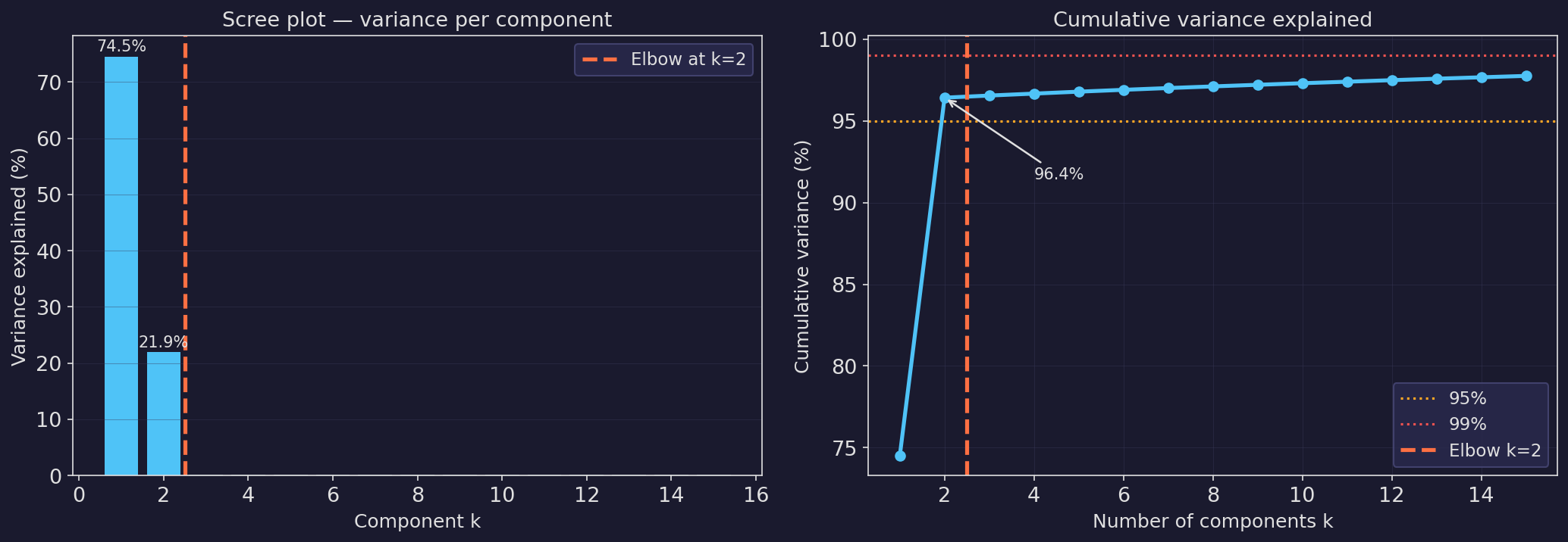
Scree plot (left) and cumulative variance plot (right) for the synthetic EELS stack. The elbow at \(k=2\) separates signal components (large bars) from noise components (flat floor).

• Plot the variance explained \(\lambda_k / \sum_k \lambda_k\) (or \(\sigma_k^2\)) for each component.
• Signal components: steeply decreasing — each one captures a large portion of variance.
• Noise components: flat floor — all roughly equal variance (noise is isotropic).

• Walk through the figure in detail. The two left bars (k=1 and k=2) are clearly taller than the rest — PC1 captures ~74.5% of variance, PC2 captures ~21.9%, and from k=3 onwards the bars are nearly equal height (the noise floor at ~0.1% each). The elbow is sharply between k=2 and k=3. Cumulative variance reaches ~96% at k=2.
• The one point to land: the noise floor is approximately flat because Poisson noise is isotropic — it adds equal variance in every direction. Signal, by contrast, is structured and anisotropic — it clusters into a few directions. The elbow is where this transition happens.
• Misconception to preempt: “the elbow is always obvious.” For real data with many phases, the elbow can be gradual. In that case, inspect the eigenspectra and score maps for PCs near the elbow — if they look like recognizable spectral features, keep them; if they look like random noise, drop them. The scree plot is a starting point, not a definitive answer.
• EM anchor: for a realistic EELS dataset from a multi-phase oxide with 5 distinct Fe/Cr/Ni environments, the elbow might be at k=6–8, not k=2. Rule of thumb: intrinsic dimensionality ≈ number of distinct chemical environments + 1–2 background components.
• Forward link: the notebook exercise asks students to construct the scree plot for their synthetic EELS stack and justify their choice of k from it. The assert in the notebook checks that choosing the correct k gives lower reconstruction error than an underfitted k=1 model.
• Transition: “Where exactly do we cut? Three rules and one check.”

Choosing K: elbow, 95 % rule and parallel analysis

• Elbow: keep the components before the curve reaches the flat noise floor.
• 95 % cumulative variance: the smallest \(K\) with \(\sum_{k\le K}\lambda_k/\sum_k\lambda_k\ge0.95\), a reasonable start for denoising.
• Parallel analysis (Horn): keep \(\lambda_k\) larger than those of random data of the same shape.
• Always inspect the eigenspectrum and score map of the last kept and the first discarded PC: structure = signal, random wiggles = noise.
• No universal \(K\): it depends on the question (compression, denoising, rare-phase discovery).

• The visual inspection check is the most important practical point. Before trusting a PCA denoising result, display the last kept PC (should be a smooth spectral shape, structured score map) and the first discarded PC (should look like noise).
• Parallel analysis replaces the subjective elbow with a statistical threshold: is this eigenvalue larger than what random noise would produce? Students should know it exists; no need to go deep.
• The one point to land: the “right” K depends on the scientific question. For compression, 95 % variance. For denoising before clustering, a larger K. For rare-phase detection, keep more components and look at residuals (pitfall 2 later).
• Misconception to preempt: “keeping 95 % of variance is always enough.” A minor phase covering 0.5 % of the area may fall below the threshold and be erased. Same for beam damage in a few pixels.
• EM anchor: in 4D-STEM grain mapping K might be 10–15; in EELS of a simple binary oxide K=2–4. Rule of thumb: number of distinct chemical environments + 1–2 background components.
• Forward link: the notebook asks students to justify K from the scree plot; its assert checks that the chosen K beats an underfitted K=1.
• Transition: “Let’s see what truncation actually does to the spectra.”

PCA denoising of EELS: reconstruction with k components

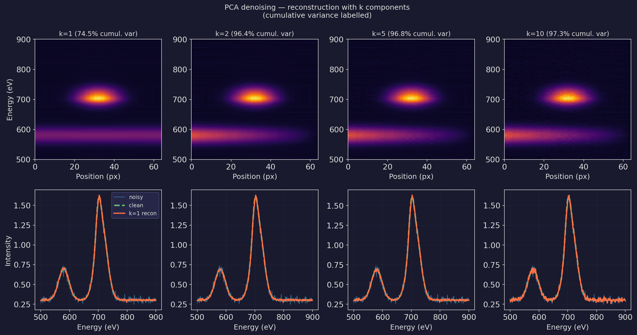
PCA reconstruction of EELS stack with k = 1, 2, 5, 10 components. Top: reconstructed spectral images; bottom: reconstructed spectra at position 24 vs noisy (blue) and clean (green dashed).

• Setup: synthetic 64-pixel × 300-channel EELS line scan, Fe-L and Cr-L components, Poisson noise → true rank 2.
• k = 1: Cr component missing → systematic error (bias).
• k = 2: recovers both components, tracks the ground truth.
• k = 5, 10: noise components added back.
• Error vs \(k\) is U-shaped; its minimum sits at the scree elbow.

• Setup (figure in the notebook, Part A): the Fe-L edge (~710 eV) is dominant in the centre of the scan, the Cr-L edge (~580 eV) at the ends; Poisson noise at scale 500 counts, i.e. realistic low-dose conditions. It mimics a grain-boundary line scan in steel, with known ground truth so we can validate.
• This is the payoff slide. The k=2 reconstruction tracks the ground truth (green dashed). k=1 is smooth but misses the Cr edge (too much truncation). k=5 and k=10 are noisier because noise components were included.
• The one point to land: there is an optimal K. Below it you lose real signal (bias); above it you add noise back. The scree elbow is the visual signal of where the optimum lives.
• Misconception to preempt: “more components = better reconstruction.” No — noise-floor components add their random variation back.
• EM anchor: Bosman et al. (2006) showed that multivariate analysis of EELS spectrum images recovers chemical and bonding (ELNES) information from noisy maps Bosman, M. et al., (2006), doi:10.1016/j.ultramic.2006.04.016. In HyperSpy, s.plot_decomposition_results() shows the same comparison.
• Forward link: the notebook assert checks that the error at k=2 is below k=1 and that adding components beyond the signal rank increases it again.
• Transition: “Why does this work so well?”

Why PCA denoising works: the subspace argument

• Signal is low-rank: if the spectrum image has \(K\) true chemical components, the clean data lies on a \(K\)-dimensional subspace of \(\mathbb{R}^D\).
• Noise is full-rank: Poisson noise adds variance in every direction equally — it spreads across all \(D\) dimensions.
• After SVD: the top \(K\) singular vectors capture the signal subspace; the remaining \(D - K\) directions are dominated by noise.
• Truncation: project onto the signal subspace (keep top \(K\)), discard the orthogonal complement (noise).
• Caveat: this assumes isotropic (equal-variance) noise. Poisson noise is signal-dependent, so the floor is not flat — hence Poisson weighting (coming up).

• This is the conceptual explanation that ties the geometry of §2–3 to the practical denoising result. The key phrase is “low-rank signal + full-rank noise.”
• The one point to land: PCA denoising is not magic — it is projection onto the signal subspace. It works because the signal is structured (low-dimensional) while the noise is unstructured (spread over all dimensions). If the signal were also spread over many dimensions, PCA would not help.
• Misconception to preempt: “PCA denoising is the best possible denoising method.” For Gaussian noise, yes (it is optimal in the Eckart–Young sense). For Poisson noise (real EELS), it is approximately optimal for high counts but suboptimal at low counts where the noise variance varies across energy channels. Anscombe transform or Poisson-matched methods can improve on it.
• EM anchor: this is why PCA denoising is so powerful for EELS: EELS spectra from a sample with \(K\) phases lie in a \(K\)-dimensional subspace regardless of how many energy channels are recorded. The “true dimensionality” is set by the chemistry, not the spectrometer resolution.
• Forward link: Week 9 (autoencoders) removes the “linearity” assumption — autoencoders can find non-linear low-dimensional structure, useful when phase boundaries curve the data manifold rather than keep it flat.
• Transition: “What do the kept components look like?”

Eigen-spectra and score maps

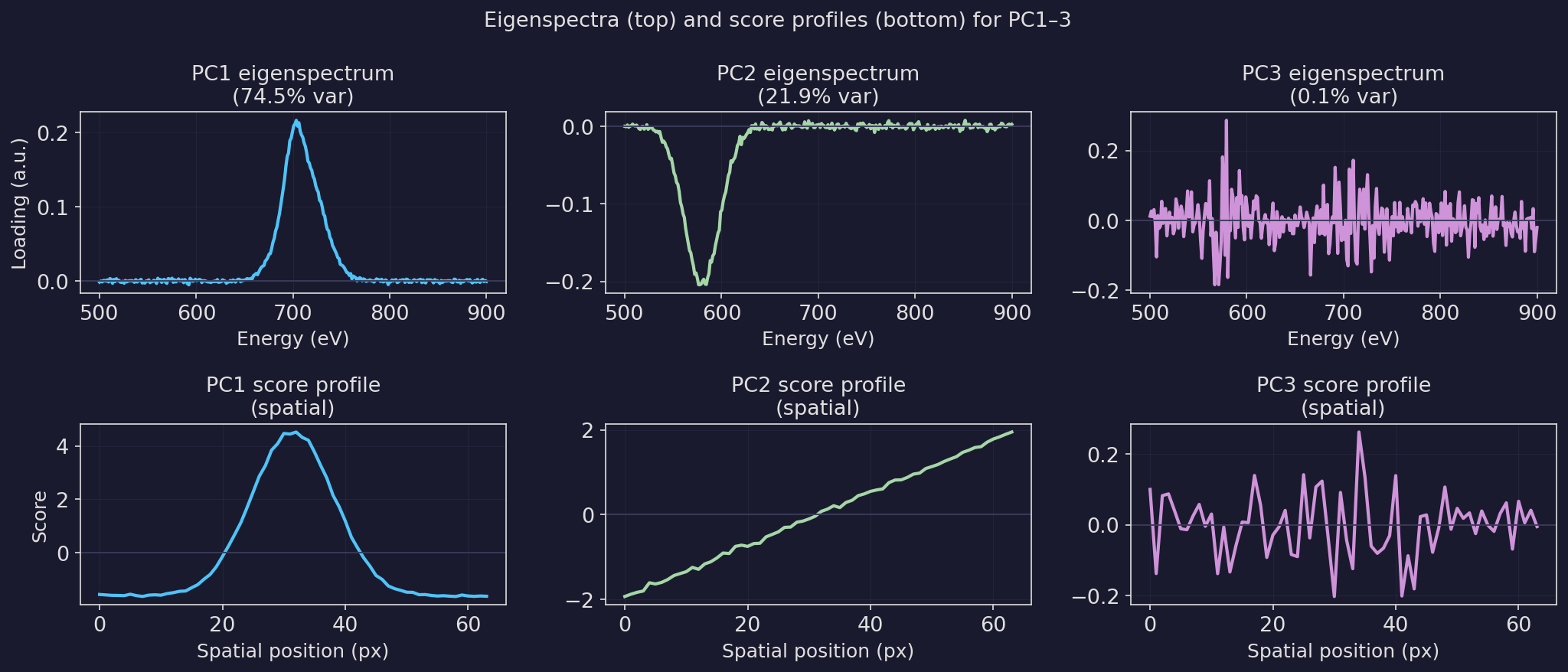
First three eigenspectra extracted from the synthetic EELS stack. PC1 captures the dominant Fe-L variation; PC2 captures the Cr-L contrast; PC3 looks like noise.

• PC1: Fe-L variation. PC2: Cr-L vs Fe-L contrast (signed). PC3+: no structure, noise.
• Scores \(c_{ik}=\mathbf{v}_k^T(\mathbf{x}_i-\bar{\mathbf{x}})\) reshaped to \((n_y,n_x)\) → score maps (eigen-micrographs).
• Eigenspectra and score maps can be negative: basis vectors, not physical spectra or concentrations.
• Reconstruction: \(\hat{\mathbf{x}}_i = \bar{\mathbf{x}} + c_{i1}\mathbf{v}_1 + c_{i2}\mathbf{v}_2\).

• Walk through each panel: PC1 has a clear peak around 710 eV (Fe-L\(_{2,3}\)). PC2 has a peak around 580 eV (Cr-L) with an anticorrelation at 710 eV. PC3 shows no recognisable structure.
• The one point to land: eigenspectra that look like spectral features are signal; random oscillations are noise. And PCA’s output is signed — it is not a phase map. That is exactly the gap the second half of the lecture closes with NMF/MCR.
• Misconception to preempt: “PC1 should look like the average Fe-L spectrum.” No — PC1 is a basis vector for the variation; the mean was removed.
• EM anchor: in real STEM-EELS, eigenspectra often resemble difference spectra between phases (oxide minus metal). Score maps are the EM analogue of eigenfaces. In 4D-STEM, PCA of diffraction patterns gives score maps with grain-orientation contrast.
• HyperSpy: s.get_decomposition_factors() = eigenspectra, s.get_decomposition_loadings() = score maps.
• Transition: “Score maps and eigenspectra come straight out of the SVD — but only if the data going in are clean. Before we unmix anything: preprocessing.”

Before any decomposition: the EELS preprocessing chain

1. Energy alignment: register every spectrum to the zero-loss peak (or a known edge onset). Drift of a fraction of an eV is enough to create fake components.
2. Spike / X-ray removal: cosmic-ray and hot-pixel spikes are rank-one outliers, and PCA will happily fit them.
3. Background subtraction: a power law \(A E^{-r}\) fitted in a pre-edge window, then extrapolated under the edge Egerton, R. F., (2011).
4. Normalisation: divide by the zero-loss or total intensity (thickness / beam-current changes). Note that this changes the noise model.
5. Poisson weighting: scale the counts so that every entry has roughly unit noise variance.
6. Only now: PCA (denoise, choose \(K\)) → NMF / MCR (interpret).

• This slide is the “garbage in dominates everything” slide of the week. Every decomposition method today is a matrix factorisation, and none of them can tell a physical component from a processing artefact.
• The one point to land: the order matters. Align before you decompose, weight before you do PCA, and always remember what each normalisation does to the noise statistics. Normalising by total counts makes the entries no longer Poisson-distributed, so weights must be computed on the raw counts.
• Misconception to preempt: “HyperSpy does all of this automatically.” s.decomposition(normalize_poissonian_noise=True) does the weighting, but alignment (align_zero_loss_peak), spike removal and background choices are your decisions, and they must be recorded in the metadata (Week 2 FAIR checklist).
• EM anchor: for core-loss EELS the edge of interest can be a few percent of the local background intensity. A 2–3% background error then dominates the extracted signal.
• NMF-specific note: after background subtraction the pre-edge region fluctuates around zero, so small negative values appear. Either clip at zero (biased), fit NMF on the raw spectra and let one component absorb the background, or model the background explicitly (the physics-guided route).
• Forward link: Week 8 (“physics decides augmentation”) and Week 12 (“forward model decides inverse method”) continue this theme. The measurement chain dictates the processing.
• Transition: “Let’s look at the two steps that most often go wrong: background and alignment.”

Power-law background and energy alignment

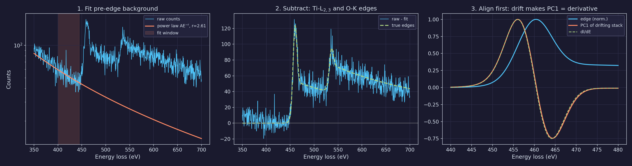
Synthetic Ti-L\(_{2,3}\) + O-K core-loss spectrum. (1) Power law fitted in a pre-edge window (log-log linear regression). (2) After subtraction the edges emerge. (3) A stack whose energy axis drifts by ±0.8 eV: its first principal component is simply the derivative \(dI/dE\) of the edge (img/make_figures.py).

• Background: \(\log I = \log A - r \log E\) is a linear least-squares fit (projection again!). Typically \(r\approx 2\)–\(6\). The fit window must be edge-free and close to the onset.
• Alignment: a rigid shift \(\delta\) adds \(\delta\cdot dI/dE\) to the spectrum (Taylor expansion). A derivative-shaped loading is therefore the fingerprint of misalignment, not of chemistry.

• Walk through the three panels left to right. Panel 1 is on a log scale: the background falls by an order of magnitude across the window, and the edges sit on top of it. Panel 2 shows that the subtracted spectrum agrees with the true edges, but only because the window was chosen sensibly. Panel 3 is the most important diagnostic of the week.
• The one point to land: a first-order Taylor expansion, \(I(E-\delta)\approx I(E)-\delta\,I'(E)\), shows that random energy shifts add a component proportional to the derivative. PCA finds that component immediately and often ranks it as PC1 or PC2. If an eigenspectrum looks like a peak derivative (a positive lobe followed by a negative lobe), suspect drift before chemistry.
• Misconception to preempt: “the background fit is a detail.” At low dose the power-law fit is itself dominated by Poisson noise, and a noisy background becomes a systematic error in every extracted edge. Cueva et al. address this with linear combinations of power laws and local background averaging, i.e. borrowing background counts from spectrally similar neighbours Cueva, Paul et al., (2012), doi:10.1017/S1431927612000244.
• EM anchor: in HyperSpy, s.remove_background(signal_range=(400., 445.), background_type='PowerLaw') does panels 1 and 2. s.align_zero_loss_peak() handles the low-loss alignment, and core-loss SIs can be shifted with the ZLP shifts from a simultaneous dual-EELS acquisition.
• Forward link: the “fit a power law in log-log space” step is exactly linear regression in transformed variables. Week 4 formalises it.
• Transition: “The last preprocessing step, weighting, is the one that decides what PCA considers signal.”

Poisson weighting before PCA

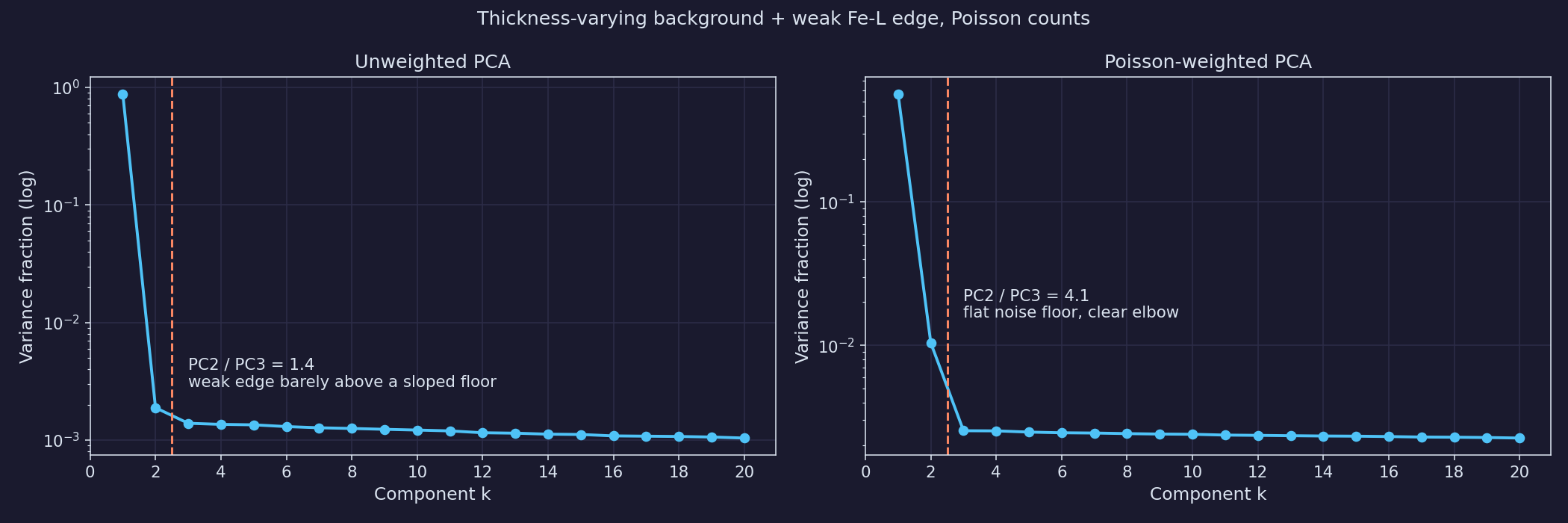
Thickness-varying background plus a weak Fe-L edge under Poisson noise. Left: unweighted PCA, where PC2 barely rises above a sloped noise floor. Right: after weighting, the noise floor is flat and the weak edge component stands out clearly (img/make_figures.py).

• Poisson counts: \(\operatorname{Var}[x_{ij}] = \mathbb{E}[x_{ij}]\). Bright channels and thick pixels dominate the variance.
• PCA = least squares, so it implicitly assumes equal-variance Gaussian noise (Week 2!).
• Weighting Keenan, Michael R. et al., (2004), doi:10.1002/sia.1657: \(\tilde{\mathbf{X}} = \mathbf{G}^{-1/2}\,\mathbf{X}\,\mathbf{H}^{-1/2}\), with \(\mathbf{G}\) = diagonal of pixel totals and \(\mathbf{H}\) = diagonal of the mean spectrum.
• After weighting, the noise is ≈ isotropic, the noise floor is flat, and the scree elbow becomes readable.
• Un-weight the reconstruction afterwards: \(\hat{\mathbf{X}} = \mathbf{G}^{1/2}\hat{\tilde{\mathbf{X}}}\mathbf{H}^{1/2}\).

• This is where Week 2’s lesson “the noise model decides the loss” returns. PCA minimises the Frobenius norm, which is the Gaussian negative log-likelihood with one shared variance. With Poisson data, high-count channels (the plasmon tail, the pre-edge background) carry more absolute variance, and PCA spends its components describing them.
• The one point to land: weighting changes which subspace is top-K. It is not cosmetic, because it decides whether a weak edge survives truncation. Compare the PC2/PC3 ratios printed in the two panels.
• Misconception to preempt: “I will just use the Anscombe transform.” That is a valid alternative (the VST from Week 2). It works per entry and does not need a rank-one model of the mean. Keenan–Kotula weighting assumes the mean matrix is approximately rank one (pixel total × mean spectrum), which is a good approximation for most spectrum images.
• EM anchor: HyperSpy’s normalize_poissonian_noise=True implements exactly this scaling. Bosman et al. showed that weighted PCA recovers ELNES bonding information that unweighted PCA loses Bosman, M. et al., (2006), doi:10.1016/j.ultramic.2006.04.016.
• Forward link: the NMF version of the same idea is to replace the Frobenius loss with the Poisson (KL) divergence. It comes in a few slides.
• Transition: “PCA has now given us a clean subspace. But its components are signed, orthogonal mixtures. How do we get phases?” (Backup: Potapov & Lubk’s weighted-PCA EDS maps, if asked about real data.)

The linear mixing model

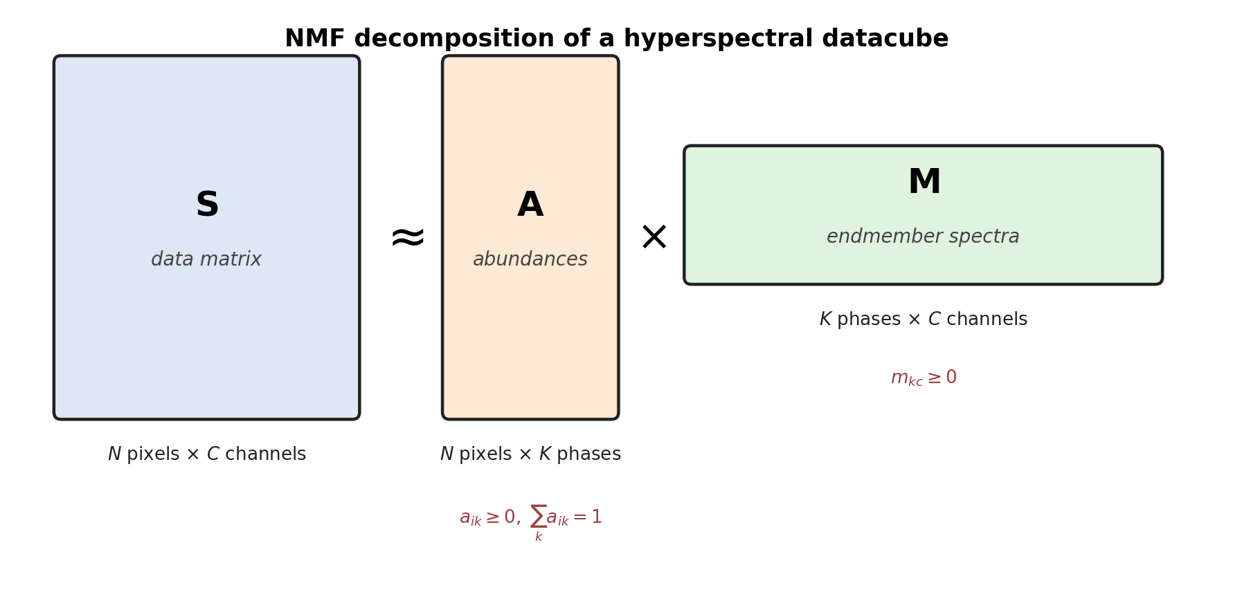
Unmixing factorises the unfolded datacube into non-negative abundances and non-negative endmember spectra (figure from ML-PC Unit 5).

• Each pixel is a mixture of pure phases (endmembers): \[\mathbf{x}_i = \sum_{k=1}^{K} a_{ik}\,\mathbf{m}_k + \boldsymbol{\varepsilon}_i,\quad a_{ik}\ge 0,\ \textstyle\sum_k a_{ik}=1\]
• Matrix form: \(\mathbf{X} \approx \mathbf{A}\mathbf{M}\) with \(\mathbf{A}\in\mathbb{R}_{\ge0}^{N\times K}\) (abundance maps) and \(\mathbf{M}\in\mathbb{R}_{\ge0}^{K\times D}\) (endmember spectra).
• Same shape as PCA (\(\mathbf{X}\approx\mathbf{T}\mathbf{V}^T\)), but with different constraints: non-negativity (+ sum-to-one) instead of orthogonality.
• Physically justified when the signal is additive: thin specimens, no strong multiple scattering or absorption.

• This slide reframes the whole week. PCA and unmixing are both rank-K factorisations of the same data matrix, and the difference lies entirely in the constraints. PCA asks for orthonormal loadings ordered by variance. Unmixing asks for spectra and abundances that could physically exist.
• The one point to land: a pixel on a phase boundary genuinely contains both phases, and its spectrum is genuinely (approximately) a linear mixture. That is why unmixing is the right model for spectrum images, and why hard clustering (K-means) is wrong on mixed pixels.
• Misconception to preempt: “linear mixing always holds.” It fails with multiple scattering (thick EELS samples: plural scattering convolves the spectrum), with EDS absorption/fluorescence in thick specimens, and with channelling. Deconvolve plural scattering (Fourier-log) first, or accept that the model is approximate.
• EM anchor: in EDS, the “endmembers” are phase spectra (including bremsstrahlung). In core-loss EELS after background removal, they are edge shapes including ELNES. In low-loss EELS, they are plasmon shapes.
• Notation: \(\mathbf{A}\) here is the MFML \(\mathbf{W}\) (activations), and \(\mathbf{M}\) is \(\mathbf{H}\) (basis). Different communities use different letters: HyperSpy calls \(\mathbf{A}\) “loadings” and \(\mathbf{M}\) “factors”, which is the opposite of the PCA convention in many textbooks. Always check shapes.
• Transition: “If we already know the endmembers, the problem is easy.”

Known endmembers: constrained least squares & the simplex

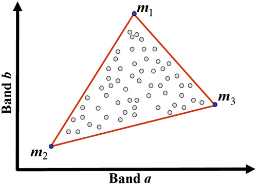
Linear mixing places every pixel inside a simplex whose vertices are the pure endmember spectra. Unmixing means finding the vertices plus each pixel’s barycentric coordinates. From Dobigeon, Nicolas et al. (2012), doi:10.1016/j.ultramic.2012.05.006.

• Known \(\mathbf{M}\) (reference spectra): solve per pixel \(\min_{\mathbf{a}_i}\|\mathbf{x}_i-\mathbf{M}^T\mathbf{a}_i\|^2\). This is projection onto the span of the references (slide “Least squares = projection”).
• Plain least squares can give negative fractions. Hence NNLS (\(\mathbf{a}\ge0\)) and FCLS (fully constrained: \(\ge0\), sum to one).
• Geometry: with sum-to-one, the pixels lie in a \((K-1)\)-dimensional simplex. The vertices are the pure phases, and mixed pixels sit inside.
• Unknown \(\mathbf{M}\), but pure pixels exist: VCA / N-FINDR search for the vertices directly.
• Unknown \(\mathbf{M}\), no pure pixels: we need a factorisation → NMF / MCR-ALS.

• Start with the easy case because it connects to the projection geometry from earlier today. Reference-spectrum fitting (e.g. HyperSpy’s model fitting with reference components, or MLLS fitting in Gatan DigitalMicrograph) is just least squares with the references as columns.
• The one point to land: draw a triangle on the board. Mark the three corners as pure TiO₂, FeO and Ni. A pixel halfway along an edge is a 50/50 mixture of two phases. A pixel in the middle contains all three. The abundances are the barycentric coordinates. This picture carries all of the unmixing theory, including rotational ambiguity (next section).
• Misconception to preempt: “negative fractions mean the fit failed.” They usually mean a missing endmember, a wrong background or misalignment. Check the residual before forcing non-negativity, because the constraint hides the symptom.
• EM anchor: Dobigeon & Brun (2012) applied Bayesian linear unmixing with exactly these simplex constraints to EELS spectrum images. They note that PCA/ICA struggle when abundances are statistically dependent, which is always the case under sum-to-one.
• Connection to the earlier PCA figure: after centering, data obeying sum-to-one lose one dimension. That is why a 3-phase mixture needs only 2 PCs (you will see PC3 = noise on the PCA-vs-NMF figure).
• Transition: “Now the real problem: we know neither the spectra nor the abundances.”

Non-negative matrix factorisation (NMF)

• Problem: given \(\mathbf{X}\ge0\), find \(\mathbf{W}\in\mathbb{R}_{\ge0}^{N\times K}\) and \(\mathbf{H}\in\mathbb{R}_{\ge0}^{K\times D}\) with \[\min_{\mathbf{W}\ge0,\,\mathbf{H}\ge0}\ \|\mathbf{X}-\mathbf{W}\mathbf{H}\|_F^2 \qquad\text{or}\qquad \min\ D_\text{KL}(\mathbf{X}\,\|\,\mathbf{W}\mathbf{H})\]
• No subtraction allowed → components can only add up. The result is a parts-based representation: peaks, edges, phases Lee, Daniel D. et al., (1999), doi:10.1038/44565.
• Frobenius loss = Gaussian likelihood; KL divergence = Poisson likelihood (up to constants). For counts, the KL loss is the principled choice (Week 2 again).
• Non-convex in \((\mathbf{W},\mathbf{H})\) jointly, but convex in each factor separately → alternating optimisation. The result depends on initialisation.
• No orthogonality and no variance ordering: components are not nested (NMF with \(K=3\) ≠ NMF with \(K=2\) plus one component).

• Lee & Seung’s 1999 Nature paper is the famous “parts of faces” result: NMF on face images gives noses, eyes and mouths as components, where PCA gives holistic eigenfaces. The reason is that without subtraction, no component can cancel another, so each must be a localised “part”.
• The one point to land: the KL divergence \(\sum_{ij} x_{ij}\log\frac{x_{ij}}{(\mathbf{WH})_{ij}} - x_{ij} + (\mathbf{WH})_{ij}\) equals, up to terms that do not depend on the model, the negative Poisson log-likelihood of \(\mathbf{X}\) given the mean \(\mathbf{WH}\). So “NMF with KL loss” is maximum-likelihood unmixing for count data, the direct analogue of Week 2’s Poisson NLL.
• Misconception to preempt: “NMF components are the pure phase spectra.” Only under additional conditions (pure pixels or pure channels, the so-called separability). In general NMF returns one of many valid factorisations. That is the rotational ambiguity pitfall later.
• Misconception 2: “choose K for NMF from its own reconstruction error.” NMF error always decreases with K. Choose K from the (weighted) PCA scree plot first, then run NMF with that K. This is the standard PCA-then-NMF pipeline.
• EM anchor: HyperSpy exposes this as s.decomposition(algorithm='NMF', output_dimension=3) (sklearn backend) and s.blind_source_separation() for ICA-type rotations.
• Transition: “How is NMF actually computed? The multiplicative update is a two-line algorithm.”

NMF by multiplicative updates

• Lee–Seung updates (Frobenius loss) Lee, Daniel D. et al., (2001), element-wise: \[\mathbf{H} \leftarrow \mathbf{H}\odot\frac{\mathbf{W}^T\mathbf{X}}{\mathbf{W}^T\mathbf{W}\mathbf{H}},\qquad \mathbf{W} \leftarrow \mathbf{W}\odot\frac{\mathbf{X}\mathbf{H}^T}{\mathbf{W}\mathbf{H}\mathbf{H}^T}\]
• Gradient descent with a per-element step size: all factors ≥ 0, so non-negativity is preserved automatically.
• The loss never increases, but convergence is slow and ends in a local minimum.
• KL version = Poisson-ML update. In practice: sklearn.decomposition.NMF(beta_loss="kullback-leibler", solver="mu"); you write the updates yourself in notebook Part D.

• Derivation sketch for the board: the gradient of \(\frac12\|\mathbf{X}-\mathbf{WH}\|^2\) w.r.t. \(\mathbf{H}\) is \(\mathbf{W}^T\mathbf{WH}-\mathbf{W}^T\mathbf{X}\), a positive part minus a negative part. Take a gradient step with element-wise step size \(\eta_{kj} = H_{kj}/(\mathbf{W}^T\mathbf{WH})_{kj}\) and the update collapses to \(H_{kj}\cdot(\mathbf{W}^T\mathbf{X})_{kj}/(\mathbf{W}^T\mathbf{WH})_{kj}\) — multiplicative, and non-negative since all terms are. Monotone decrease follows from a majorisation argument.
• KL update: \(\mathbf{H}\leftarrow\mathbf{H}\odot\frac{\mathbf{W}^T(\mathbf{X}/\mathbf{WH})}{\mathbf{W}^T\mathbf{1}}\).
• The one point to land: a special case of the gradient descent of Week 4, with a clever learning rate. The first learning algorithm of the course that students can write by hand in five lines.
• sklearn call used in the notebook: NMF(n_components=3, init="nndsvda", beta_loss="kullback-leibler", solver="mu", max_iter=1000, random_state=0); W = nmf.fit_transform(X) gives abundances (N, K), H = nmf.components_ spectra (K, D).
• Misconception to preempt: “multiplicative updates are the best solver.” Simple and robust, but slow. Coordinate descent (sklearn default solver='cd') or HALS are faster for the Frobenius loss; for KL, mu is the standard sklearn option.
• Practical warning: a zero entry stays zero forever. Initialise strictly positive (NNDSVDa fills zeros with the mean).
• Transition: “Let’s compare what PCA and NMF return on the same data.”

PCA vs NMF on a synthetic 3-phase spectrum image

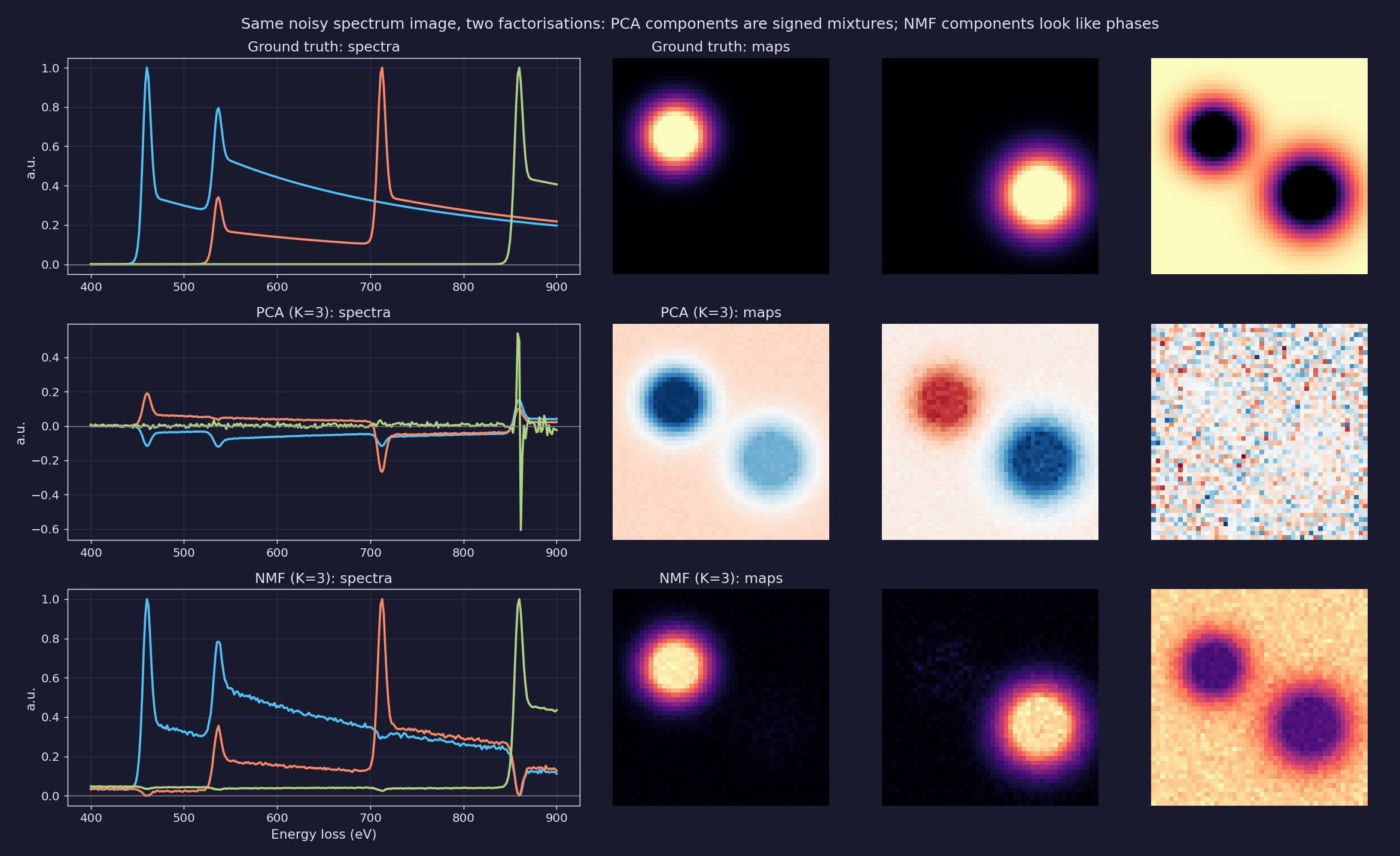
Top: ground-truth endmembers (TiO\(_2\)-like, FeO-like, Ni) and abundance maps. Middle: PCA with \(K=3\). The components are signed difference spectra, the maps have positive and negative lobes, and PC3 is pure noise (sum-to-one removes one dimension after centering). Bottom: NMF with \(K=3\) recovers phase-like spectra and non-negative maps, with small artefacts at the edge onsets (img/make_figures.py, same data as the notebook).

• Walk row by row. The ground truth consists of two particles in a Ni matrix, with the O-K edge shared by both oxides. The PCA spectra (middle) are signed and look like “oxide minus metal” and “Ti-oxide minus Fe-oxide” differences. The maps are blue/red, so neither a spectrum nor a map is physically interpretable on its own. The third PC is noise, because with sum-to-one the centered data have rank K−1 = 2.
• The one point to land: PCA and NMF span (almost) the same subspace. The reconstructions are nearly identical, but the basis inside that subspace is different. PCA picks the orthogonal, variance-ordered basis, and NMF picks a non-negative one. Choosing a basis is a modelling decision, not a data fact.
• Look at the NMF spectra: the shared O-K edge is split correctly between the two oxides, but there are small dips at 710 eV and 855 eV where edges overlap. These are ambiguity artefacts, which set up the rotational-ambiguity slide.
• Misconception to preempt: “NMF found the truth, so NMF is right.” Here it works because (a) there are nearly pure pixels in every phase and (b) the endmembers have regions of zero intensity (before their onsets). Both conditions make the factorisation close to unique. Remove them and NMF drifts.
• EM anchor: this is the exact result the notebook asks students to reproduce and quantify (spectral correlation and abundance RMSE against ground truth after Hungarian matching of components).
• Transition: “NMF has one constraint. Chemometrics adds more: MCR-ALS.”

MCR-ALS: multivariate curve resolution

• Model: \(\mathbf{X} = \mathbf{C}\mathbf{S}^T + \mathbf{E}\), with \(\mathbf{C}\) = concentrations (maps) and \(\mathbf{S}\) = pure spectra Juan, Anna de et al., (2014).
• Alternating least squares:
  1. Initialise \(\mathbf{S}\) (purest pixels, PCA + varimax, or reference spectra).
  2. \(\mathbf{C} \leftarrow \arg\min_{\mathbf{C}}\|\mathbf{X}-\mathbf{C}\mathbf{S}^T\|^2\) subject to the constraints.
  3. \(\mathbf{S} \leftarrow \arg\min_{\mathbf{S}}\|\mathbf{X}-\mathbf{C}\mathbf{S}^T\|^2\) subject to the constraints.
  4. Repeat until the relative change in the residual is < \(10^{-6}\).
• Each half-step is an ordinary (constrained) least-squares problem, i.e. a projection.
• NMF = MCR with non-negativity only. MCR adds closure, unimodality, known spectra, selectivity / local rank.

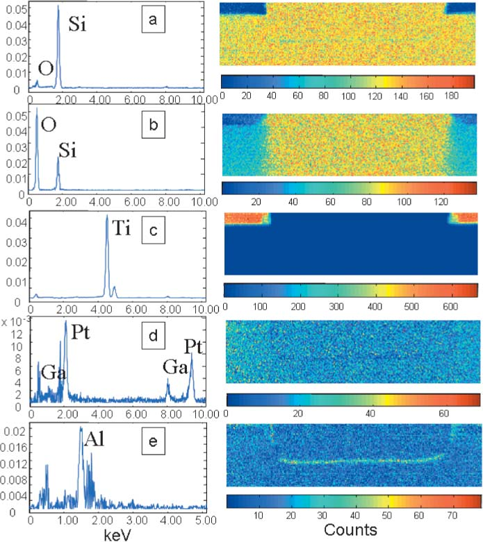
MCR of a STEM-EDS spectrum image of a microelectronics interface: pure-component spectra (O, Si, Ti, Pt/Ga, Al) and their abundance maps, extracted from the raw datacube. From Kotula, Paul G. et al. (2006), doi:10.1017/S1431927606060636.

• MCR-ALS comes from analytical chemistry (chromatography, reaction monitoring), where de Juan & Tauler developed the constraint toolbox. Kotula & Keenan at Sandia brought it to STEM-EDS in the early 2000s. It is why MCR/PCA were the production default in EDS labs decades before deep learning.
• The one point to land: the constraints are the science. Non-negativity alone leaves a band of valid answers. Closure (fractions sum to one), unimodality (a diffusion profile has one maximum), a known reference spectrum or a region where only one phase is present are physical statements that shrink the band.
• Misconception to preempt: “MCR-ALS is just NMF with extra steps.” Mathematically yes, and that is the point. The extra steps turn a generic factorisation into a physically constrained one. Plain NMF has no knowledge of the physics. MCR lets you inject it.
• Implementation detail: the simplest non-negativity step is least squares followed by clipping negatives to zero. It is crude but widely used. Proper NNLS per pixel is more accurate but slower. The notebook’s optional MCR-ALS cell uses clipping plus closure.
• EM anchor (figure): the Ga/Pt component is the FIB-implanted Ga and the protective Pt cap. MCR isolates this contamination into its own component instead of letting it contaminate the chemistry. Read every component, including the boring ones.
• Transition: “Which brings us to the pitfalls. Why is a factorisation not unique, and how do we notice when it is lying?” (Backup: NMF-aided deep-mantle STEM-EDXS case study.)

Pitfall 1: rotational ambiguity of NMF / MCR

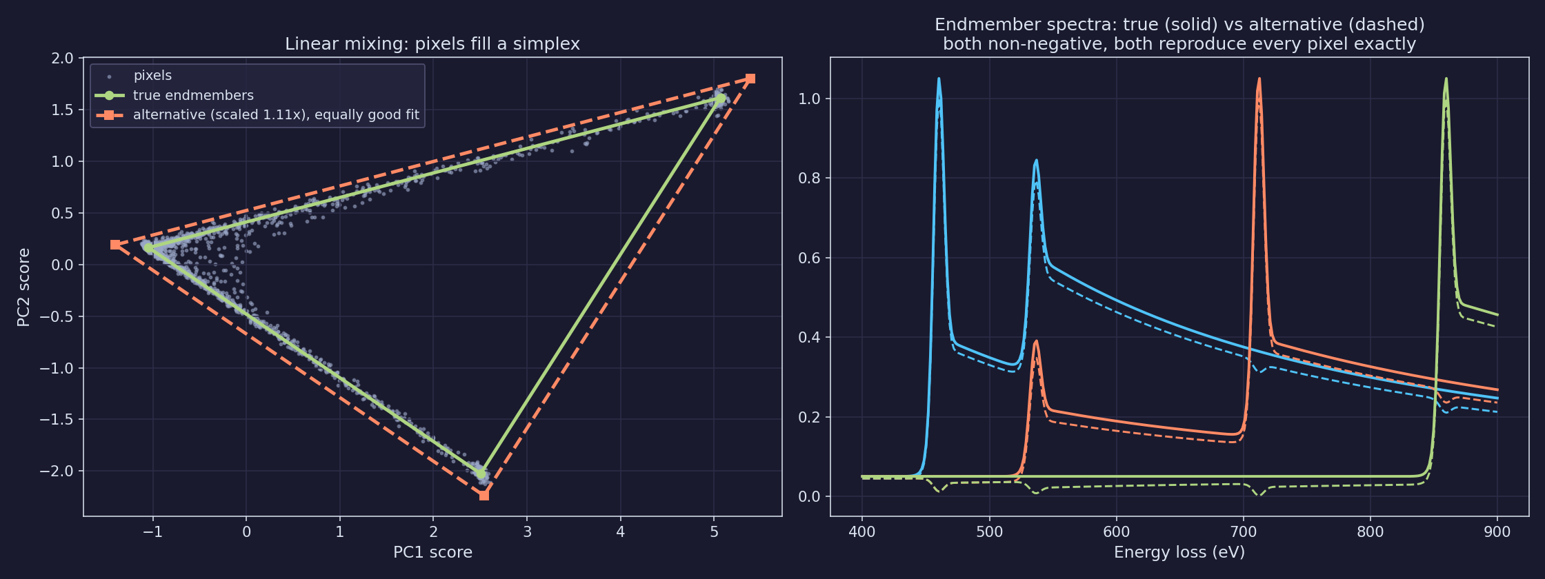
Pixels of the 3-phase SI projected onto PC1–PC2 fill a triangle (simplex). An enlarged triangle (dashed) with non-negative vertex spectra reproduces every pixel exactly, with different spectra and different abundances (img/make_figures.py).

• For any invertible \(\mathbf{T}\): \(\mathbf{X} = \mathbf{C}\mathbf{S}^T = (\mathbf{C}\mathbf{T})(\mathbf{T}^{-1}\mathbf{S}^T)\), with identical fit.
• Non-negativity only rules out some \(\mathbf{T}\). It leaves a feasible band of solutions.
• Geometrically: any simplex that encloses the data and has non-negative vertices is a valid answer.
• Symptoms: endmembers change between restarts, or converge consistently to spectra with dips / copies of other phases. Consistency ≠ correctness.
• Remedies: closure, known spectra, pure pixels / selectivity, physics-guided endmembers. Always report your constraints.
• PCA is unique (up to sign) only because it imposes orthogonality.

• Board derivation: write \(\mathbf{X} = \mathbf{C}\mathbf{S}^T\), insert \(\mathbf{T}\mathbf{T}^{-1}\) in the middle, and regroup. The fit is unchanged. For PCA we remove this freedom by demanding orthonormality and variance ordering, which is why PCA is unique (up to sign) and NMF is not.
• The one point to land (figure): the true triangle and the enlarged dashed triangle both contain all pixels and both have non-negative vertex spectra, so both are perfectly valid NMF solutions. The dashed spectra (right panel) are the true spectra with a bit of the other phases subtracted, which is exactly the “dips at other phases’ edges” artefact seen in the NMF row two slides ago.
• Misconception to preempt: “a better optimiser will find the true solution.” No. All points in the feasible band have the same loss, so it is an identifiability problem, not an optimisation problem. Only more information (constraints, priors) can resolve it.
• War story (from the MCR literature): two groups publish “the pure phase spectrum” of the same material, and the spectra differ. Both are valid points in the feasible band, and neither group reported its constraints.
• Practical diagnostic: run NMF from 10 random initialisations. If the endmembers change qualitatively, the band is wide, so add constraints or report the range. Tools such as MCR-BANDS compute the feasible band explicitly.
• Exam-weight: state rotational ambiguity and name two constraints that reduce it.
• Transition: “The second pitfall concerns PCA itself, specifically what truncation throws away.”

Pitfall 2: PCA truncation bias and the rare phase

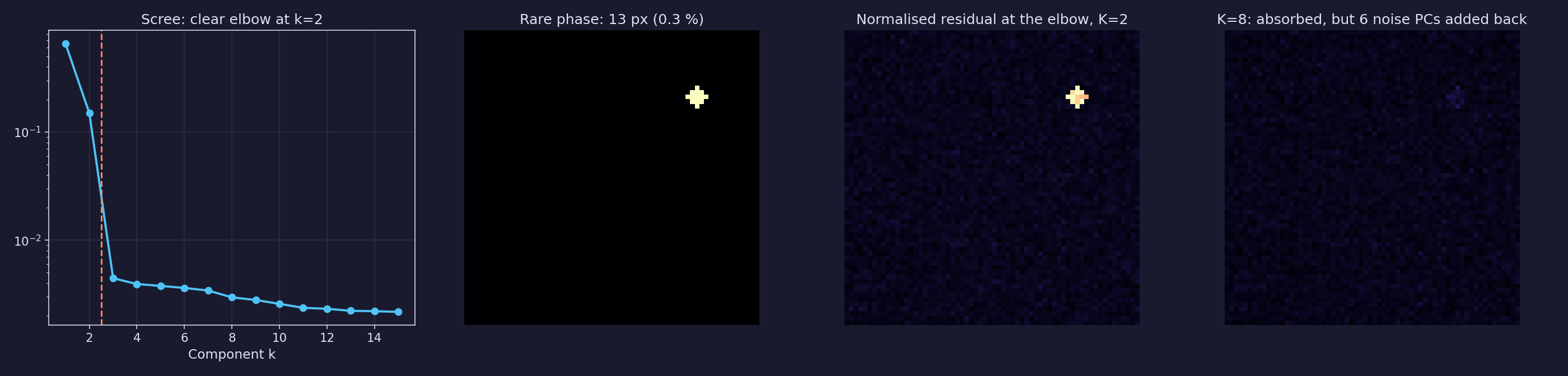
A rare phase occupying 13 pixels (0.3 %) is invisible in the scree plot (elbow at \(k=2\)). The Poisson-normalised residual at \(K=2\) shows it as a spatially coherent hot spot, and only at \(K\approx8\) is it absorbed, together with six noise components (img/make_figures.py).

• Truncation keeps variance, not importance. A rare or dilute phase contributes little variance and falls below the noise floor, so it is projected away.
• The noisy estimate of the loadings is itself biased. PCA-filtered maps can be precise and biased at once Lichtert, Stijn et al., (2013), doi:10.1016/j.ultramic.2012.10.001. With poor peak-to-background, PCA filtering creates artefacts Cueva, Paul et al., (2012), doi:10.1017/S1431927612000244.
• Diagnostic: always inspect the residual map \(\|\mathbf{x}_i-\hat{\mathbf{x}}_i\|^2/\hat{\mathbf{x}}_i\). It must look like spatially uncorrelated noise.

• The one point to land: “looks clean” ≠ “is correct”. The denoised reconstruction at K=2 looks perfect and the scree plot gives a textbook elbow, yet a real phase has been erased. The only place it survives is the residual, and a Poisson-normalised residual map makes it jump out.
• Why K=8 is not the answer: the rare phase is spread over several noise-level components, so you would add back 6 components of noise to recover 13 pixels. The right approach is to detect it in the residual and then analyse that region specifically (local PCA, targeted fitting, or simply the raw summed spectrum of those pixels).
• Lichtert & Verbeeck (2013) is the key cautionary paper: PCA noise filtering of atomic-resolution EELS maps can bias fitted parameters while making the precision look better than the Cramér–Rao bound. A tighter error bar around the wrong value is worse than an honest wide one.
• Misconception to preempt: “so never denoise.” Denoise when the features of interest are common (matrix phase quantification). For discovery (rare phases, dopants, defects), work with residual maps or the raw data. Different question, different tool.
• EM anchor: dopant segregation to a grain boundary is the classic rare-phase case. The boundary is a few pixels wide and its variance is tiny, and PCA will happily smooth it away.
• Forward link: Week 9 revisits this with anomaly detection on autoencoder reconstruction errors, which applies the same residual logic to a non-linear model.
• Transition: “Let me put the methods side by side before we turn to ill-conditioning.”

Choosing the decomposition: a decision table

Question	Method	Constraint	Unique?	Watch out for
How many things vary? Denoise	PCA / SVD (weighted)	orthogonal, variance-ordered	yes (± sign)	truncation bias, rare phases, needs weighting
Which phases, known references	NNLS / FCLS	\(\mathbf{a}\ge0\), \(\sum a=1\)	yes	missing endmember → biased fractions
Which phases, unknown spectra	NMF (Frobenius / KL)	\(\mathbf{W},\mathbf{H}\ge0\)	no	rotational ambiguity, init, choose \(K\) from PCA
+ physical prior knowledge	MCR-ALS / physics-guided NMF	+ closure, unimodality, known spectra	≈ with enough constraints	constraints must be true
Discrete phases, no mixing	K-means / GMM (Week 9)	hard / soft labels	no (init)	mixed pixels at boundaries
Curved manifolds, shifting peaks	Autoencoders (Week 9)	learned non-linear	no	interpretability, validation

• This table is the practical summary of the second half of the lecture. It is worth copying into the miniproject report template.
• The one point to land: PCA and unmixing are not competitors. The standard pipeline is: preprocess → weighted PCA to denoise and choose K → NMF/MCR with that K for interpretation → residual maps to check what was lost.
• Misconception to preempt: “clustering gives phase maps.” Only when the phases are spatially separated and spectrally distinct (e.g. the duplex-steel low-loss EELS case in ML-PC Unit 5). Otherwise every boundary pixel is wrong, and unmixing is the right tool.
• Forward link: Week 9 covers the last two rows. Constrained autoencoders (softmax bottleneck + linear decoder) are literally NMF-style unmixing learned by gradient descent.
• Transition: “One practical warning that bridges to next week: correlated features and ill-conditioning.”

Ill-conditioning: when correlated features cause trouble

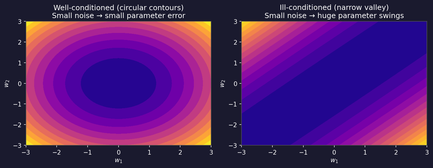
Loss landscape: well-conditioned problem (circular contours, left) vs ill-conditioned problem (narrow valley, right). Small noise → large parameter swing in the ill-conditioned case.

• Condition number \(\kappa = \sigma_\text{max}/\sigma_\text{min}\) — ratio of largest to smallest singular value.
• Well-conditioned: \(\kappa \approx 1\) (circular contours). Ill-conditioned: \(\kappa \gg 1\) (narrow valley).
• Cause: highly correlated features → data matrix nearly singular → small \(\sigma_\text{min}\) → large \(\kappa\).
• Effect: a tiny change in the data produces huge, unstable swings in the estimated parameters Murphy, Kevin P., (2012).
• Cures: standardise features, project onto the top PCs, or Ridge (Week 4).

• Walk through the loss landscape figure: the circular contours mean that moving in any direction costs you the same loss — you can locate the minimum reliably. The narrow valley means the loss is nearly flat along the valley floor — many parameter combinations give almost the same loss, but they correspond to wildly different physical predictions.
• The one point to land: \(\kappa \gg 1\) means the matrix amplifies small errors (noise, rounding) by a factor of \(\kappa\). If \(\kappa = 10^4\), floating-point noise at the \(10^{-16}\) level becomes \(10^{-12}\) errors in the solution — usually fine. But noise at the \(10^{-3}\) level (real measurement noise) becomes errors of order \(10\), which is catastrophic.
• Misconception to preempt: “ill-conditioning means the model is wrong.” No — the model can be perfectly specified but the data matrix is ill-conditioned. The solution is not a different model but a different computation: use SVD (which can detect and handle small singular values) instead of direct inversion.
• EM anchor: in EDS mapping of an alloy with Fe and Mn close in energy, the two elemental maps are highly correlated because the Fe-K\(\alpha\) and Mn-K\(\alpha\) peaks overlap. Directly fitting both peaks simultaneously creates a near-singular regression matrix. SVD-based pseudo-inverse or regularisation (Ridge) is the standard fix.
• Forward link: in Week 4, ridge regression adds \(\lambda\mathbf{I}\) to the normal equations, which lifts all eigenvalues by \(\lambda\) and eliminates ill-conditioning. This is the standard cure.
• Transition: “Before we close: what are the limits of linear methods, and what comes next?” (Backup: FeNi EDS example and a condition-number diagnostic checklist.)

Limits of linear methods

• Linearity: PCA, NMF and MCR all assume \(\mathbf{X}\approx\) (maps) × (spectra). Peak shifts (strain, valence), peak-shape changes (ELNES), plural scattering and EDS absorption bend the data cloud off the flat subspace / simplex.
• Noise, identifiability, rare features: weight or use KL; add constraints; inspect residual maps (see the pitfalls).
• These limits motivate Week 9: autoencoders learn non-linear low-dimensional representations, and constrained autoencoders learn NMF-style unmixing.

• Frame the limits positively: knowing where a method fails is as important as knowing where it works. Linear decomposition is the right first tool for any spectral dataset.
• The one point to land: every limit on this slide has a specific diagnostic. Curvature appears as many components with smooth, structured eigenspectra (a peak shift shows up as a derivative-shaped loading, as we saw). Noise-model mismatch appears as a sloped noise floor. Ambiguity appears as restart-dependence. Rare features appear as structured residuals.
• Misconception to preempt: “if PCA fails, I should use deep learning.” Not necessarily. Weighting fixes the noise problem, NMF/MCR fix the non-negativity problem, alignment fixes the shift problem, and constraints fix the ambiguity problem. Reach for autoencoders only for genuine non-linearity, and choose the simplest tool that handles the specific failure mode.
• EM anchor: a solid solution whose edge onset shifts with composition forms a curved 1-D manifold. PCA needs 2–3 components (edge + derivative + curvature), whereas a 1-D non-linear latent captures it.
• Forward link: an autoencoder with linear activations and MSE loss exactly recovers the PCA subspace. With a softmax bottleneck and a non-negative linear decoder it becomes an unmixing model. Week 9 builds both.
• Transition: “Let’s summarise.”

Summary

• Data matrix: spectrum image \((n_y,n_x,D)\) → \(\mathbf{X}\in\mathbb{R}^{N\times D}\), rows = pixels. Every method today factorises \(\mathbf{X}\approx\) maps × spectra.
• SVD / PCA: rotate–stretch–rotate; singular values² ∝ variance; truncation = projection onto the signal subspace (Eckart–Young). Unique, but components are signed.
• Scree plot & denoising: signal = steep head, noise = flat floor. Too few components → bias, too many → noise.
• Preprocessing: align → remove spikes → power-law background → normalise → Poisson-weight → decompose.
• NMF / MCR-ALS: non-negativity (+ closure, …) gives phase-like spectra and maps. Multiplicative updates / alternating LS. KL loss = Poisson likelihood.
• Pitfalls: rotational ambiguity (report constraints, check restarts), truncation bias (inspect residual maps), ill-conditioning (κ = σ_max/σ_min).

• Use this slide as the verbal recap. Ask two students to explain one bullet each in their own words, focusing on the preprocessing and pitfalls bullets, since they are new.
• The one point to land: the same factorisation shape appears everywhere, and only the constraints change. Orthogonality gives PCA, non-negativity gives NMF, physical constraints give MCR, and a learned non-linear decoder gives an autoencoder (Week 9).
• Transition: “Here are the statements you must be able to reproduce in the exam.”

Must-know takeaways

1. PCA = SVD of the centered data matrix; \(\sigma_k^2/(N-1)\) is the variance along PC \(k\); truncating at \(K\) is the best rank-\(K\) approximation (Eckart–Young).
2. PCA denoises because the signal is low-rank and the noise is full-rank; choose \(K\) where the scree plot meets the noise floor.
3. PCA is least squares, i.e. it assumes equal-variance Gaussian noise. Poisson-weight counts before PCA.
4. EELS preprocessing order: align → background (power law) → normalise → weight → decompose. A derivative-shaped loading signals misalignment.
5. NMF: \(\mathbf{X}\approx\mathbf{WH}\), \(\mathbf{W},\mathbf{H}\ge0\) gives a parts-based, physically plausible basis; KL-NMF = Poisson maximum likelihood.
6. NMF / MCR are not unique: \(\mathbf{CS}^T = (\mathbf{CT})(\mathbf{T}^{-1}\mathbf{S}^T)\). Constraints (closure, known spectra, selectivity) reduce the ambiguity.
7. Truncation removes low-variance, not unimportant, signal. Always inspect residual maps.

• These seven statements are exactly what goes into _shared/mustknow_parts/week03.md (plus a couple of related ones). The exam will ask for at least one of them in the form “explain why…”.
• The one point to land: statements 3, 6 and 7 are the ones students most often get wrong. Rehearse them.
• Transition: “Next week: the projection geometry becomes regression.”

Looking ahead: Week 4

• Topic: “Regression, optimisation & honest validation”.
• Linear regression as projection, building directly on today’s least-squares geometry.
• Gradient descent, SGD and Adam: loss landscapes and why ill-conditioning (today’s \(\kappa\)) makes optimisation slow.
• Ridge and Lasso: systematic cures for ill-conditioning, and their geometry.
• Honest validation: train/val/test, k-fold, GroupKFold by specimen. Also why every preprocessing step (scaling, PCA, feature selection) must be fitted inside the training fold.

• Keep this light. It is a teaser, not a lecture. The key promise: after Week 4, students can fit a regularised linear model to EM-derived features and report an honest estimate of how well it generalises.
• The one point to land: the multiplicative NMF update was a gradient step with a clever learning rate. Week 4 makes gradient descent the central algorithm, and today’s condition number tells you how hard the landscape is.
• Forward link to the leakage demo: the Week 4 notebook shows that selecting features on the full dataset before splitting invents a positive R² from pure noise. Fitting a scaler or PCA before the split leaks less dramatically, but it is the same mistake: fit every step of this PCA pipeline inside the training fold.
• Transition: “Here is what to do this week.”

Self-study this week

• Notebook: notebooks/week03_pca_nmf_eels.ipynb, “PCA vs NMF on a synthetic spectrum image”.
  • Part A: PCA denoising of an EELS line scan (SVD, scree plot, U-shaped error curve).
  • Part B: a 3-phase 2-D spectrum image with Poisson noise and a known ground truth.
  • Part C: PCA vs NMF: match components to the ground truth, quantify spectral correlation and abundance error.
  • Part D: write multiplicative updates yourself; break NMF by removing pure pixels (rotational ambiguity); optional MCR-ALS with closure.
• Goal: be able to explain why PCA components are not phases and when NMF can be trusted.

Open in Colab

CPU only, < 5 min end-to-end. Uses NumPy, SciPy, matplotlib and scikit-learn.

• Distribute the Colab link now. The notebook runs end-to-end in well under five minutes on a CPU.
• The one point to land: Part C’s quantitative comparison (correlation of recovered vs true spectra, RMSE of abundance maps) is the habit we want. Never judge a decomposition by eye alone when a ground truth or a physical check exists.
• Misconception to preempt: “the notebook is just the lecture again in code.” Part D asks students to implement the multiplicative update by hand and to break NMF: remove the pure pixels and NMF converges, consistently across restarts, to wrong endmembers that fit the data as well as the truth. That experience makes rotational ambiguity concrete, and shows that restart-consistency is not proof of correctness.
• Miniproject link: teams working on spectral data should treat this notebook as a template for their pipeline (preprocess → weighted PCA → NMF → residual check).
• Transition: “See you next week for regression and validation.”

Continue

• ← Previous: Unit 02 — Learning from EM data: signal formation, noise & loss
• → Next: Unit 04 — Regression, optimisation & honest validation
• All courses

Backup slides

Material for questions and self-study; not part of the 90-minute lecture path.

Weighting and truncation in practice

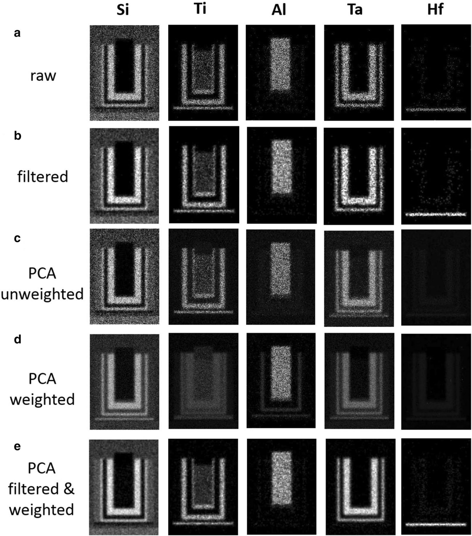
STEM-XEDS element maps: raw → filtered → PCA unweighted → PCA weighted → PCA filtered & weighted. Weighting plus the right truncation separates a clean map from a destroyed one. From Potapov, Pavel et al. (2019), doi:10.1186/s40679-019-0066-0.

• EDS counts are even sparser than EELS counts (often < 1 count per channel per pixel). Without weighting, PCA mainly models the bremsstrahlung.
• Potapov & Lubk derive the optimal truncation rank from the noise statistics. It beats eyeballing the scree elbow Potapov, Pavel et al., (2019), doi:10.1186/s40679-019-0066-0.
• Recipe: weight → PCA → choose \(K\) where the eigenvalues leave the noise floor (flat after weighting) → reconstruct → un-weight.
• Record weighting, \(K\) and the software version. Otherwise the map is not reproducible (Week 2 FAIR).

• Walk down the columns of the figure: the unweighted PCA row still shows noise-like texture in the minority elements, while the weighted row is clean. The difference comes entirely from the scaling step, since the algorithm is otherwise identical.
• The one point to land: “denoise with PCA” is not one method. It is a family of choices (weighting, K, spatial pre-filtering), and each choice changes the result. Report them.
• Misconception to preempt: “a fixed rule like keep 5 components is fine for all samples.” A facility-wide fixed K can discard a dilute dopant on one sample and keep noise on another. K is a per-dataset decision.
• EM anchor: this paper is the standard reference for anyone doing PCA on STEM-EDS maps. Students who do the spectral miniproject should read its method section.
• Transition: “PCA has now given us a clean subspace. But its components are signed, orthogonal mixtures. How do we get phases?”

Case study: NMF-aided phase unmixing of STEM-EDXS

• Sample: lower-mantle assemblage from a diamond-anvil cell: bridgmanite, ferropericlase, Ca-perovskite, doped with trace Nd/Sm/U Chen, Hui et al., (2024), doi:10.1016/j.ultramic.2024.113981.
• Problem: the phases share X-ray lines and intermix below the pixel scale. The per-pixel EDXS is far too noisy for trace elements.
• Pipeline: NMF (3 components) → phase spectra + abundance maps → constrained least-squares refinement → quantification.
• Result: trace Sm detected in ferropericlase down to tens of ppm.
• Next step: physics-guided NMF, where endmembers are built from X-ray emission theory and fitted with a Poisson loss Teurtrie, Adrien et al., (2024).

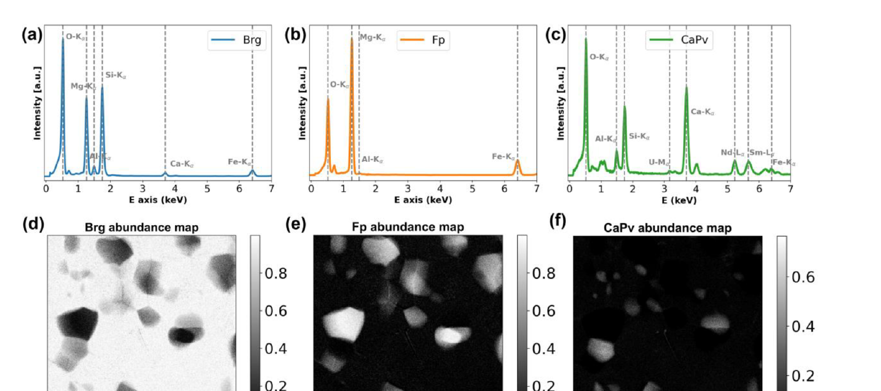
Recovered phase spectra of bridgmanite, ferropericlase and Ca-perovskite after NMF-aided unmixing (a–c), and the corresponding abundance maps (d–f). From Chen, Hui et al. (2024), doi:10.1016/j.ultramic.2024.113981.

• Why this is the right case study: clustering (K-means / GMM) fails here because the phases overlap spectrally and spatially. A hard cluster map would be wrong on nearly every mixed pixel. NMF pools the counts of all pixels belonging to a phase into one clean endmember spectrum, which is how a per-pixel-noisy measurement becomes a trace-element measurement.
• The one point to land: the benefit of unmixing is statistical. The endmember spectrum is estimated from thousands of pixels, so its SNR is far higher than that of any single pixel. This is the same “exploit redundancy” argument as PCA denoising, but in a physically interpretable basis.
• Physics-guided NMF (Teurtrie et al., the espm Python package): instead of learning arbitrary non-negative spectra, parameterise each endmember by elemental concentrations times theoretical X-ray line shapes plus a bremsstrahlung model. Fit with the Poisson (KL) loss. This greatly reduces rotational ambiguity, because the spectra can no longer take arbitrary shapes.
• Misconception to preempt: “a black-box NMF result is publishable.” Chen et al. validate against known phase compositions and refine the abundances with constrained least squares. The NMF step is a starting point, not the answer.
• Transition: “Which brings us to the pitfalls. Why is a factorisation not unique, and how do we notice when it is lying?”

The covariance matrix: where geometry meets statistics

• Covariance matrix of centered data: \(\mathbf{S} = \frac{1}{N-1}\tilde{\mathbf{X}}^T\tilde{\mathbf{X}} \in \mathbb{R}^{D \times D}\).
• Entry \(S_{ij}\) = covariance between energy channels \(i\) and \(j\); \(S_{ii}\) = variance of channel \(i\).
• Geometry: the level set \(\mathbf{x}^T\mathbf{S}^{-1}\mathbf{x} = 1\) is an ellipsoid whose axes are the eigenvectors of \(\mathbf{S}\) with lengths \(\propto \sqrt{\lambda_k}\) (eigenvalues).
• PCA = align the coordinate axes with the ellipsoid axes: rotate to the eigenbasis of \(\mathbf{S}\), where features are uncorrelated.
• In EM: off-diagonal entries of \(\mathbf{S}\) are large when two energy channels always increase or decrease together (e.g. Fe-L23 channels are correlated because they all belong to the same edge).

• The covariance matrix slide is the bridge between the abstract “directions of maximum variance” idea and the concrete eigenvector calculation. The ellipsoid picture is the geometric key: the long axis of the data ellipsoid is PC1.
• The one point to land: the shape of the covariance ellipsoid is exactly what PCA extracts. A thin, elongated ellipsoid means the data is highly structured and low-dimensional (good for PCA); a spherical ellipsoid means the data is isotropic (PCA helps little — all directions have equal variance).
• Misconception to preempt: “the covariance matrix is \(N \times N\)” (number of observations squared). It is \(D \times D\) (number of features squared). For EELS data with 1024 channels and 4096 pixels, the covariance matrix is 1024×1024, not 4096×4096. This is why PCA is feasible even for huge numbers of pixels.
• EM anchor: in EELS, correlated energy channels are the norm because each element contributes a characteristic edge shape that spans many channels. The covariance matrix of EELS spectra is block-diagonal, with each block corresponding to an element’s edge region.
• Forward link: SVD of the centered data matrix gives exactly the eigenvectors of \(\mathbf{S}\) without ever forming \(\mathbf{S}\) explicitly — which is important because forming \(\mathbf{S}\) is computationally expensive and can be numerically unstable for large \(D\).
• Transition: “Now the big tool: SVD as a geometric picture.”

Matrices as geometric transformations

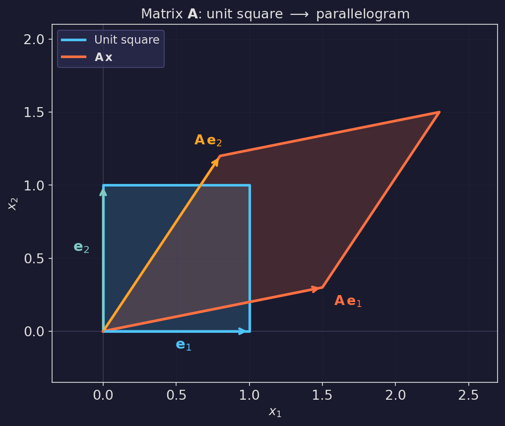
A \(2\times2\) matrix applied to the unit square: rotates, stretches, and shears — the unit square (blue) becomes a parallelogram (orange).

• A matrix \(\mathbf{A}\) maps every vector \(\mathbf{x}\) to a new vector \(\mathbf{y} = \mathbf{Ax}\).
• Geometrically: \(\mathbf{A}\) rotates, stretches, and (for non-symmetric \(\mathbf{A}\)) shears space.
• The data matrix \(\mathbf{X} \in \mathbb{R}^{N \times D}\): \(N\) spectra (rows), each with \(D\) energy channels (columns).
• One row = one spectrum = one point in \(\mathbb{R}^D\).
• Convention for this week: observations in rows, features in columns.

• The unit-square picture is the classic: take the four corners of the unit square, apply \(\mathbf{A}\) to each corner, watch the square become a parallelogram. This encodes the full action of the matrix geometrically.
• The one point to land: a matrix is not just a 2-D spreadsheet — it is a machine that reshapes space. Understanding what kind of reshaping it does (rotation? stretch? compression?) is the key to understanding PCA and SVD.
• Misconception to preempt: “the data matrix has \(D\) rows (features) and \(N\) columns (observations).” Different fields use different conventions. In this course: observations (spectra, pixels, samples) are rows; features (energy channels, pixel values) are columns. Always check shape with .shape.
• EM anchor: for an EELS spectrum image of shape (64, 64, 1024), you reshape the first two axes to get the data matrix \(\mathbf{X}\) of shape (4096, 1024) — 4096 spectra, each with 1024 energy channels. This is the input to PCA.
• Forward link: the column space of \(\mathbf{X}\) (the span of all spectra) is the subspace PCA is searching for a compact basis for.
• Transition: “When we talk about ‘dimensions’ of EM data, what do we mean precisely?”

Why correlated features cause ill-conditioning in EM

• Scenario: two EDS channels (Fe-K\(\alpha\) at 6.4 keV and Ni-K\(\alpha\) at 7.5 keV) both increase with sample thickness in an FeNi alloy.
• Forming a regression matrix from both channels → two nearly parallel column vectors → near-singular \(\mathbf{X}^T\mathbf{X}\) → high \(\kappa\).
• PCA as a cure: PCA rotates to the principal directions. In the new basis, the directions are uncorrelated by construction (orthogonal). The PCA-transformed data matrix has no correlated columns.
• Practical rule: if your condition number is \(> 10^3\) and you are fitting a linear model, standardise your features (subtract mean, divide by std) and consider PCA pre-processing or Ridge regularisation.
• Fitting with highly correlated features gives wildly uncertain coefficients even when the prediction accuracy looks fine.

• The key insight: high prediction accuracy with correlated features does not mean the coefficients are physically meaningful. The model found one combination of coefficients that works, but many other combinations work equally well (the loss valley is flat). Any perturbation of the data changes which combination is selected.
• The one point to land: “correct predictions, wrong coefficients” is a genuine failure mode. If you are using regression coefficients as physical descriptors (e.g., “the model says the Fe contribution is 0.7”), you need well-conditioned data for those numbers to be interpretable.
• Misconception to preempt: “I can check if my features are correlated by looking at the correlation matrix.” Yes — but the correlation matrix shows pairwise correlation. SVD shows the effective dimensionality of the full feature matrix, including higher-order redundancies. High condition number with moderate pairwise correlations is common.
• EM anchor: in 4D-STEM strain mapping, the lattice parameters \(a\) and \(c\) of a hexagonal crystal are often correlated in strained regions. Directly fitting both can produce unstable strain maps; using PCA-reduced diffraction pattern features as inputs avoids this.
• Forward link: Week 4 introduces regularisation (Ridge, Lasso) as the systematic cure for ill-conditioning. PCA pre-processing (projecting onto the well-conditioned principal components) is an alternative.
• Transition: “Before we close: what are the limits of linear methods, and what comes next?”

Ill-conditioning: a quick diagnostic

• Check condition number: np.linalg.cond(X) — if \(> 10^6\), you have a serious problem.
• Variance–inflation factor (VIF): for each feature, regress it on all others. High \(R^2\) → high VIF → high collinearity.
• Standardise first: features on vastly different scales (counts vs kV vs nm) create artificial ill-conditioning. Always subtract the mean and divide by the standard deviation before linear modelling.
• PCA as pre-processing: project features onto the first \(K\) principal components (choose \(K\) to drop near-zero singular values). The resulting \(K\) features are guaranteed to be uncorrelated.
• Ridge regularisation (Week 4): adds \(\lambda\mathbf{I}\) to \(\mathbf{X}^T\mathbf{X}\), lifting all eigenvalues above \(\lambda\) — quick fix when you want to keep all features.

• This is a practical toolbox slide. Give students a decision tree: (1) check condition number; (2) if high, check for correlated features; (3) standardise; (4) if still high, use PCA pre-processing or Ridge. Each step has a specific NumPy/sklearn call.
• The one point to land: standardisation (subtract mean, divide by std) is the first step in any linear model pipeline when features have different physical units. Skipping it is one of the most common beginner errors — it creates artificial ill-conditioning that has nothing to do with the actual physics.
• Misconception to preempt: “standardisation distorts the physical meaning of the features.” Standardisation changes scale but not relative variation. The regression coefficients after standardisation are in units of “standard deviations of the feature per unit target” — which is a meaningful, interpretable scale for comparing feature importances.
• EM anchor: in compositional analysis, if one feature is “Ti content in at%” (range 0–100) and another is “peak position in eV” (range 460–470), the scale difference is 100× — enough to create artificial ill-conditioning when both are used in a regression together.
• Forward link: Week 4 presents Ridge regression and introduces the explicit regularisation \(\lambda\). The geometric interpretation: Ridge replaces the sharp SVD truncation with a soft shrinkage of all singular values, which is smoother and often more practical.
• Transition: “Let’s close with the limits of linear methods and what we build toward.”

References

Pattern recognition and machine learning, Christopher M. Bishop.

EELS elemental mapping with unconventional methods i. Theoretical basis: Image analysis with multivariate statistics and entropy concepts, Ultramicroscopy, Patrick Trebbia & Nicolas Bonnet.

Mapping chemical and bonding information using multivariate analysis of electron energy-loss spectrum images, Ultramicroscopy, M. Bosman, M. Watanabe, D. T. L. Alexander, & V. J. Keast https://doi.org/10.1016/j.ultramic.2006.04.016.

Electron energy-loss spectroscopy in the electron microscope, R. F. Egerton.

Data processing for atomic resolution electron energy loss spectroscopy, Microscopy and Microanalysis, Paul Cueva, Robert Hovden, Julia A. Mundy, Huolin L. Xin, & David A. Muller https://doi.org/10.1017/S1431927612000244.

Accounting for Poisson noise in the multivariate analysis of ToF-SIMS spectrum images, Surface and Interface Analysis, Michael R. Keenan & Paul G. Kotula https://doi.org/10.1002/sia.1657.

Spectral mixture analysis of EELS spectrum-images, Ultramicroscopy, Nicolas Dobigeon & Nathalie Brun https://doi.org/10.1016/j.ultramic.2012.05.006.

Learning the parts of objects by non-negative matrix factorization, Nature, Daniel D. Lee & H. Sebastian Seung https://doi.org/10.1038/44565.

Algorithms for non-negative matrix factorization, Advances in Neural Information Processing Systems, Daniel D. Lee & H. Sebastian Seung.

Multivariate curve resolution (MCR). Solving the mixture analysis problem, Analytical Methods, Anna de Juan, Joaquim Jaumot, & Romà Tauler.

Application of multivariate statistical analysis to STEM x-ray spectral images: Interfacial analysis in microelectronics, Microscopy and Microanalysis, Paul G. Kotula & Michael R. Keenan https://doi.org/10.1017/S1431927606060636.

Statistical consequences of applying a PCA noise filter on EELS spectrum images, Ultramicroscopy, Stijn Lichtert & Jo Verbeeck https://doi.org/10.1016/j.ultramic.2012.10.001.

Machine learning: A probabilistic perspective, Kevin P. Murphy.

Optimal principal component analysis of STEM XEDS spectrum images, Advanced Structural and Chemical Imaging, Pavel Potapov & Axel Lubk https://doi.org/10.1186/s40679-019-0066-0.

Non-negative matrix factorization-aided phase unmixing and trace element quantification of STEM-EDXS data, Ultramicroscopy, Hui Chen, Farhang Nabiei, James Badro, Duncan T. L. Alexander, & Cécile Hébert https://doi.org/10.1016/j.ultramic.2024.113981.

From STEM-EDXS data to phase separation and quantification using physics-guided NMF, arXiv preprint arXiv:2404.17496, Adrien Teurtrie, Nathanaël Perraudin, Thomas Holvoet, Hui Chen, Duncan T. L. Alexander, Guillaume Obozinski, & Cécile Hébert.