Data Science for Electron Microscopy
Week 4: Regression, gradient descent & honest validation

Prof. Dr. Philipp Pelz

FAU Erlangen-Nürnberg

Institute of Micro- and Nanostructure Research

FAU Logo IMN Logo CENEM Logo ERC Logo Eclipse Logo

Recap: where we left off

  • Week 3: linear algebra & PCA — SVD, score maps, eigenspectra.
  • You can now compress a 50 000-spectrum EELS dataset into a handful of components and plot a scree plot.
  • Key geometric insight: least-squares = projection of the target vector onto the column space of \(\mathbf{X}\).
  • Gap: projection gives the optimal weights analytically, but only when we can invert \(\mathbf{X}^T\mathbf{X}\). For large or non-linear problems we need an iterative approach — gradient descent.
  • Gap #2: fitting a model well on training data is not the same as fitting it honestly. We will spend the second half of today on that distinction.

Today’s questions

  • Why does a model trained on EM crops from one specimen fail on crops from a new specimen? Because crops from the same specimen are correlated — training on them while testing on others measures memorisation, not generalisation.
  • How do we find model parameters without inverting a matrix? Gradient descent: follow the slope of the loss surface downhill, one small step at a time.
  • Road map: prediction = loss minimisation (3) · MSE / MAE / Huber & noise (5) · loss landscape & GD picture (4) · learning rate (3) · SGD → Adam, intuition only (6) · overfitting & bias–variance (4) · train/val/test (4) · K-fold CV (3) · data leakage in EM — the crop-vs-specimen trap (6) · regression & segmentation metrics (4) · limits + Week 5 preview (2).
  • Self-study: notebooks/week04_leakage_demo.ipynb — fit a regressor two ways and watch the honest score drop.

Prediction = minimising a loss

  • Dataset: \(\mathcal{D} = \{(\mathbf{x}_i, y_i)\}_{i=1}^N\) — each \(\mathbf{x}_i\) is a feature vector, \(y_i\) is the target.
  • Predictor: \(\hat{y}_i = f_{\mathbf{w}}(\mathbf{x}_i)\) — parameterised by weights \(\mathbf{w}\).
  • Loss: \(L(\hat{y}_i, y_i)\) — a scalar that scores how wrong prediction \(i\) is.
  • Empirical risk (what we minimise): \(\hat{R}(\mathbf{w}) = \dfrac{1}{N}\sum_{i=1}^{N} L(f_{\mathbf{w}}(\mathbf{x}_i),\, y_i)\).
  • Goal: \(\hat{\mathbf{w}} = \arg\min_{\mathbf{w}} \hat{R}(\mathbf{w})\).

Every supervised learning algorithm is a choice of loss + a choice of optimiser.

The linear model & the normal equations

  • Linear predictor: \(\hat{y} = \mathbf{w}^T \mathbf{x} + b = \mathbf{w}^T \mathbf{x}\) (absorb \(b\) into \(\mathbf{w}\)).
  • MSE loss for linear regression: \(\hat{R}(\mathbf{w}) = \tfrac{1}{N}\|\mathbf{X}\mathbf{w} - \mathbf{y}\|^2\).
  • Analytic solution (Normal equations): \(\hat{\mathbf{w}} = (\mathbf{X}^T\mathbf{X})^{-1}\mathbf{X}^T\mathbf{y}\).
  • Geometric reading (Week 3): \(\hat{\mathbf{y}} = \mathbf{X}\hat{\mathbf{w}}\) is the projection of \(\mathbf{y}\) onto the column space of \(\mathbf{X}\).
  • Problem: inverting \(\mathbf{X}^T\mathbf{X}\) fails when \(D\) is large or features are correlated (\(\kappa(\mathbf{X}^T\mathbf{X}) \gg 1\)).

Enter gradient descent — an iterative alternative that never inverts anything.

What is the gradient?

  • The gradient \(\nabla_\mathbf{w} \hat{R}(\mathbf{w})\) is a vector pointing in the direction of steepest ascent of the loss surface.
  • Key insight: moving opposite to the gradient (steepest descent) reduces the loss (at least locally).
  • First-order Taylor: \(\hat{R}(\mathbf{w} - \eta \nabla \hat{R}) \approx \hat{R}(\mathbf{w}) - \eta \|\nabla \hat{R}\|^2 < \hat{R}(\mathbf{w})\) for small \(\eta > 0\).
  • For MSE linear regression: \(\nabla_\mathbf{w} \hat{R} = \tfrac{2}{N}\mathbf{X}^T(\mathbf{X}\mathbf{w} - \mathbf{y})\) — a matrix-vector product, no inversion needed.

Gradient descent: take the gradient, step opposite to it, repeat.

Gradient descent — the update rule

  • Update rule: \(\mathbf{w}_{t+1} = \mathbf{w}_t - \eta\,\nabla_\mathbf{w}\hat{R}(\mathbf{w}_t)\).
  • Initialisation: start at some \(\mathbf{w}_0\) (typically small random values or zeros).
  • Repeat until the loss stops decreasing (convergence criterion) or a budget is exhausted.
  • For MSE linear regression: closed form for the gradient — \(\nabla_\mathbf{w}\hat{R} = \tfrac{2}{N}\mathbf{X}^T(\mathbf{Xw} - \mathbf{y})\).
  • For any differentiable model: backpropagation (Week 5) computes the gradient automatically.
  • The key insight: we only ever need first-order information (the gradient). No matrix inverses, no second-order terms.

MSE — the default regression loss

  • \(L_{\text{MSE}}(\hat{y}, y) = (\hat{y} - y)^2\) — penalises errors quadratically.
  • Smooth, convex bowl landscape — gradient descent’s ideal setting.
  • Probabilistic identity: minimising MSE over the dataset = maximum-likelihood estimation (MLE) assuming iid Gaussian residuals \(\varepsilon \sim \mathcal{N}(0, \sigma^2)\) Bishop, Christopher M., (2006).
  • In EM: correct when your noise is additive Gaussian (readout noise, Johnson noise). For Poisson-dominated low-dose data, use Poisson NLL instead (Week 2 recap).

MSE punishes large residuals heavily — one bad crop can dominate the loss.

MAE and Huber — robust alternatives

MSE, MAE, and Huber loss as functions of the residual \(r = \hat{y}-y\). MSE grows quadratically; MAE linearly; Huber switches at \(|r|=\delta\).
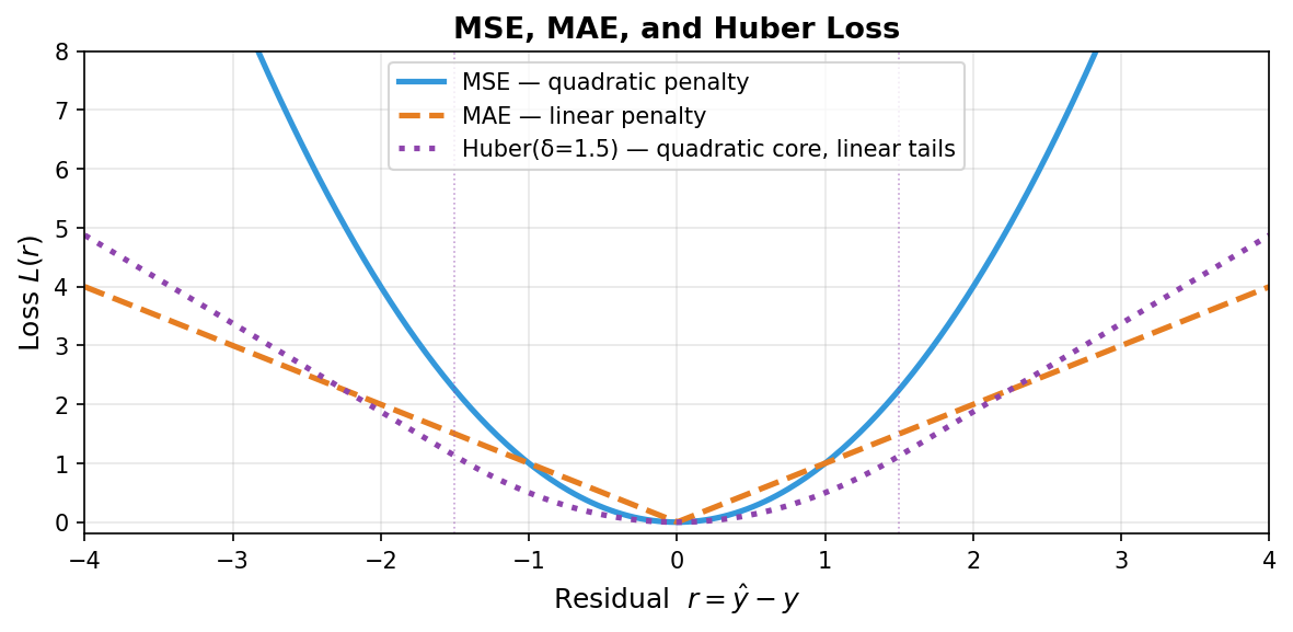
  • MAE: \(L = |\hat{y} - y|\) — linear penalty, robust to outliers. Probabilistic identity: MLE under Laplacian residuals. Caveat: non-differentiable at zero → sub-gradient methods needed.
  • Huber: quadratic inside \(|r| \le \delta\), linear outside. Best of both: smooth optimisation where residuals are small, robust to spikes. Standard tool when most EM crops are clean but occasional detector artefacts occur.
  • Rule of thumb: start with MSE; switch to Huber if residual plots show heavy tails.

The loss landscape — a bowl in weight space

Gradient descent on an ill-conditioned 2D loss bowl. Left: learning rate too large — steps overshoot and bounce back and forth, then diverge. Right: good learning rate — smooth monotone descent to the minimum.
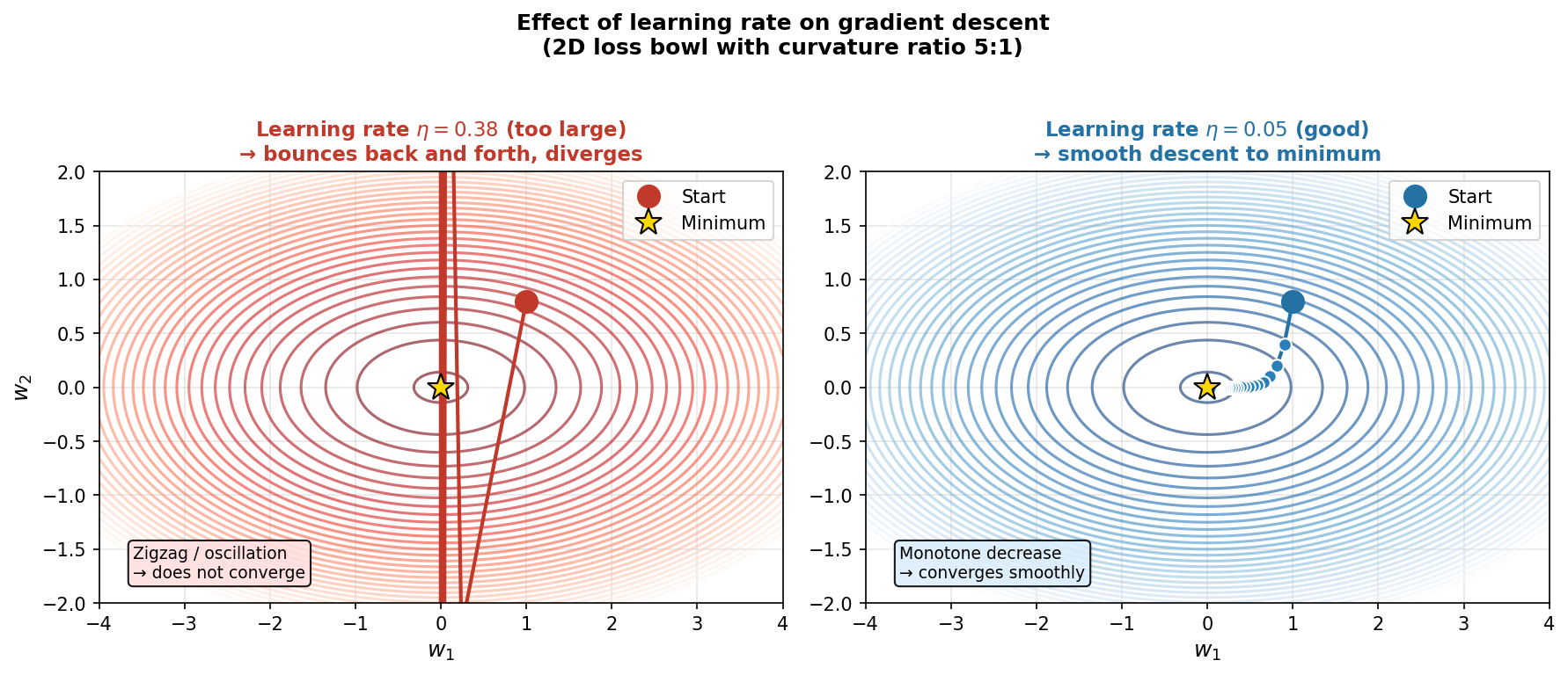
  • Loss landscape: the surface \(\hat{R}(\mathbf{w})\) over all possible weight vectors \(\mathbf{w}\).
  • For MSE linear regression: a convex bowl — one global minimum, no local traps.
  • Gradient descent update: \(\mathbf{w}_{t+1} = \mathbf{w}_t - \eta\,\nabla_\mathbf{w}\hat{R}(\mathbf{w}_t)\).
  • \(\eta\) = learning rate — the step size along the negative gradient.
  • The contour lines are level sets of the loss; GD crosses them at right angles (steepest descent).

Why the loss landscape shape matters

  • Convex (MSE, Ridge): one bowl, one minimum — GD will find it.
  • Non-convex (any neural network): many local minima, saddle points, plateaus.
  • For non-convex losses, GD finds a minimum, not necessarily the best one.
  • Practical message for EM: linear models trained with MSE are convex → any GD run converges to the same answer. Neural networks (Week 5) require careful initialisation and momentum to avoid bad local minima.
  • Saddle points (equal numbers of upward and downward curvatures): gradient is zero but no minimum — GD stalls unless there is noise (SGD rescues this, next section).

Learning rate — too small, just right, too large

Effect of learning rate on 1D gradient descent: too small (slow), just right (smooth), too large (diverges).
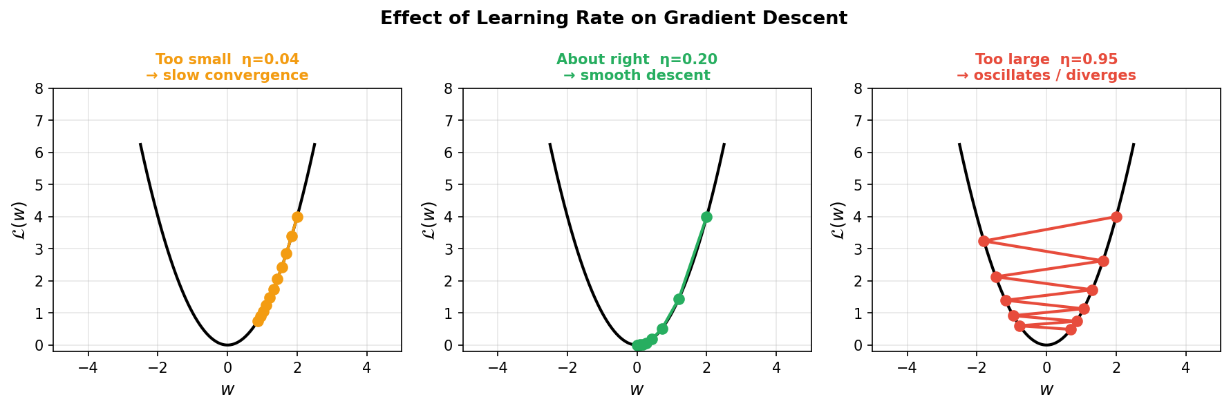
  • Too small (\(\eta \ll 1/L\), \(L\) = Lipschitz constant of gradient): correct direction but tiny steps → converges in theory, but takes too long in practice.
  • About right: loss decreases monotonically; convergence in tens to hundreds of steps.
  • Too large (\(\eta > 2/L\)): overshoots the minimum repeatedly → oscillates or diverges.
  • Rule of thumb: start at \(\eta = 0.01\)\(0.1\), monitor the loss curve, reduce if it bounces.

Learning rate schedules

  • Constant: \(\eta_t = \eta_0\) — simplest, works if \(\eta_0\) is well chosen.
  • Exponential decay: \(\eta_t = \eta_0\,e^{-\lambda t}\) — fast early, conservative late.
  • Step decay: \(\eta_t = \eta_0 \cdot \gamma^{\lfloor t/s \rfloor}\) — halve every \(s\) epochs.
  • Reduce on plateau: halve \(\eta\) when the loss has not improved for \(k\) epochs. Default in many EM projects.
  • Why decay helps: large \(\eta\) early → explore; small \(\eta\) late → fine-tune near the minimum.

When can GD get stuck?

  • Local minima — non-convex losses (all neural networks) have multiple dips. GD finds a minimum, not necessarily the best one.
  • Saddle points — gradient is zero but no minimum exists; GD stalls exactly there.
  • Plateaus — gradient is near zero over a wide region; GD crawls.
  • Vanishing gradients — for deep networks, gradients can shrink exponentially with depth (Week 5 details). The update becomes negligible far from the output.
  • Good news: for problems with wide flat minima (most modern over-parameterised networks), many local minima have similar loss values. SGD’s noise helps escape narrow sharp minima and saddle points naturally.

Stochastic gradient descent (SGD)

  • Full GD cost: \(\nabla\hat{R} = \tfrac{1}{N}\sum_i \nabla L_i\)\(\mathcal{O}(N)\) per step. Expensive for \(N \sim 10^6\).
  • SGD: pick one sample \(i\) at random; use \(\nabla L_i(\mathbf{w})\) as the gradient estimate.
  • Key property: \(\mathbb{E}_i[\nabla L_i] = \nabla\hat{R}\) — unbiased estimate of the true gradient.
  • Cost: \(\mathcal{O}(1)\) per step — dramatic speedup.
  • Behaviour: noisy steps, but rapid early progress; bounces near the minimum.
  • SGD’s noise helps escape saddle points — a genuine advantage over full GD on non-convex surfaces.

Minibatch SGD — the practical default

  • Minibatch of size \(b\): average the gradient over \(b\) randomly selected samples. \[\mathbf{w}_{t+1} = \mathbf{w}_t - \frac{\eta}{b}\sum_{i \in \mathcal{B}_t}\nabla L_i(\mathbf{w}_t)\]
  • Why \(b\) matters:
    1. Variance reduction: \(\text{Var}(\text{gradient estimate}) \propto 1/b\) — larger \(b\) = smoother steps.
    2. Vectorisation: modern GPUs process \(b\) samples in parallel almost for free (\(b = 32\)\(256\)).
  • Typical \(b\): 32, 64, 128 — hardware-aligned powers of 2.
  • This is the default training loop for every neural network you will use from Week 5 onwards.

Momentum — the physics intuition

  • Problem: SGD on an elongated bowl zigzags across the steep dimension while crawling along the flat one.
  • Momentum idea: accumulate a “velocity” vector that persists across steps — like a ball rolling downhill: \[\mathbf{v}_t = \beta\,\mathbf{v}_{t-1} + \nabla L(\mathbf{w}_{t-1}), \qquad \mathbf{w}_t = \mathbf{w}_{t-1} - \eta\,\mathbf{v}_t\]
  • \(\beta \approx 0.9\): 90% of previous velocity is preserved. Consistent gradient directions accumulate; oscillating directions cancel.
  • Effect: smoother, faster convergence on ill-conditioned landscapes.

1

Adam — the go-to optimiser

Optimizer trajectories on an ill-conditioned quadratic bowl (elongation ratio 20:1): GD zigzags across the steep dimension; SGD+momentum is visibly smoother; Adam reaches the minimum in far fewer steps.
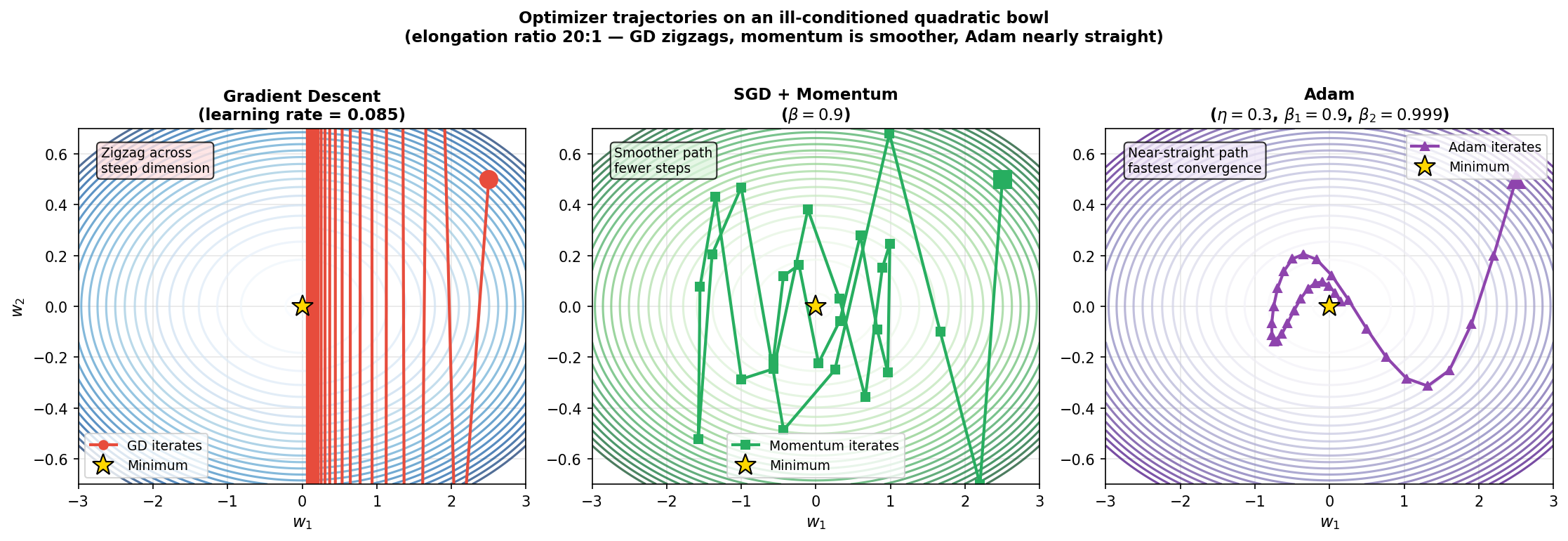
  • Adam: tracks both the gradient (momentum term \(\hat{\mathbf{v}}_t\)) and the squared gradient (adaptive scaling \(\hat{\mathbf{s}}_t\)): \[\mathbf{w}_t \leftarrow \mathbf{w}_{t-1} - \frac{\eta\,\hat{\mathbf{v}}_t}{\sqrt{\hat{\mathbf{s}}_t} + \epsilon}\]
  • Adaptive scaling: each parameter gets its own effective learning rate — large for slowly-updated parameters, small for fast ones.
  • Typical hyperparameters: \(\eta = 0.001\), \(\beta_1 = 0.9\) (momentum), \(\beta_2 = 0.999\) (RMS), \(\epsilon = 10^{-8}\).
  • For most EM projects: use Adam at its default settings unless you have a specific reason to change them.

Optimiser comparison — a visual summary

Optimiser Per-step cost Adaptive \(\eta\)? Momentum? Typical use
Full GD \(\mathcal{O}(N)\) No No Tiny datasets, convex
SGD \(\mathcal{O}(1)\) No No Rarely used bare
Minibatch SGD \(\mathcal{O}(b)\) No Optional Many DL papers
SGD + Momentum \(\mathcal{O}(b)\) No Yes (\(\beta \approx 0.9\)) Fine-tuned vision models
Adam \(\mathcal{O}(b)\) Per-param Yes Default for most EM projects
  • Rule: start with Adam at its defaults. Switch to SGD+momentum only if you have a specific reason (e.g. matching a published training recipe, or if Adam converges to a sharp minimum that generalises poorly).
  • Not covered here: AdaGrad, RMSProp, AdamW, Nesterov — all first-order, all variations on the same theme.

Overfitting and underfitting

Three polynomial fits to the same noisy data: degree 1 (underfit), degree 3 (good), degree 12 (overfit). The true signal is \(\sin(x)\).
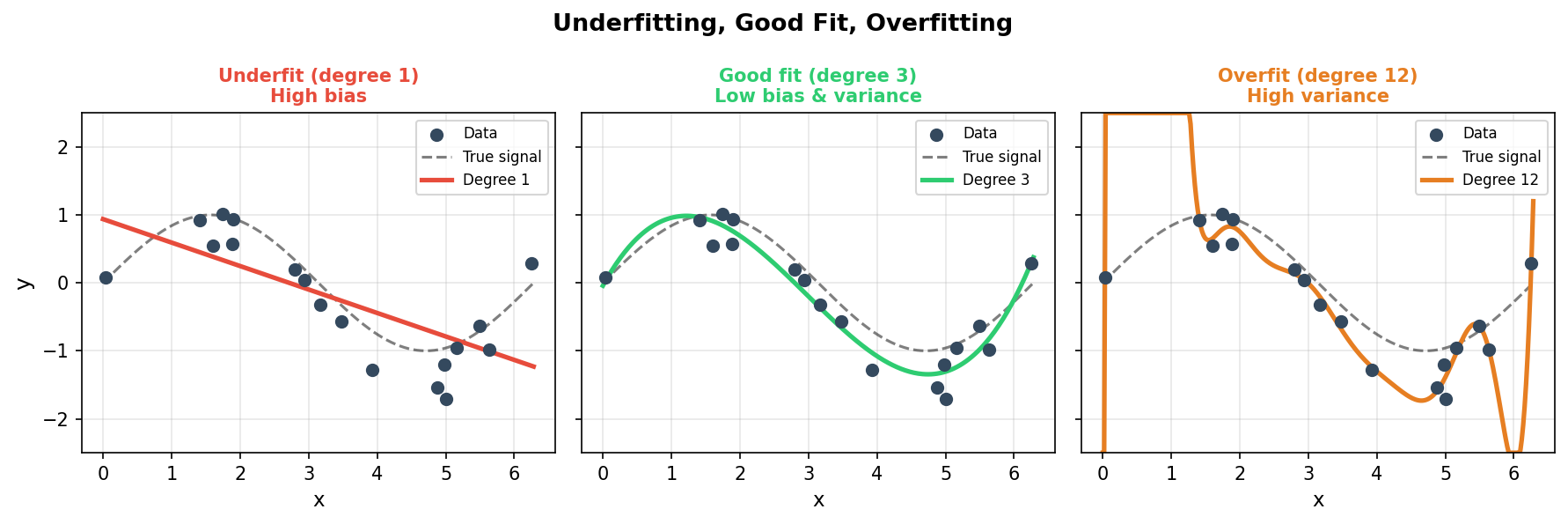
  • Underfit (high bias): model too simple — cannot capture the pattern. Training and test errors are both high.
  • Good fit (balanced): training error ≈ test error; the model captures the signal, not the noise.
  • Overfit (high variance): model too flexible — memorises training noise. Training error ≈ 0, test error ≫ 0.
  • In EM: a degree-12 polynomial fitted to 18 noisy data points passes through every point but predicts wildly on new samples.

Bias–variance decomposition

  • For squared-error loss, the expected test error decomposes as Bishop, Christopher M., (2006): \[\mathbb{E}\bigl[(\hat{y} - y)^2\bigr] = \underbrace{(\mathbb{E}\hat{y} - y)^2}_{\text{Bias}^2} + \underbrace{\text{Var}(\hat{y})}_{\text{Variance}} + \underbrace{\sigma^2}_{\text{Noise floor}}\]
  • Bias: systematic error — how far the average prediction is from the truth (underfitting).
  • Variance: sensitivity to the training set — how much the prediction changes across different training sets (overfitting).
  • Noise \(\sigma^2\): irreducible — set by the physics and detector (recall Week 2: shot noise, readout noise).
Regime Bias Variance Cure
Underfit High Low More flexible model / features
Good fit Low Low
Overfit Low High More data, fewer parameters, regularisation

The training error vs test error diagnostic

  • Diagnostic rule: | Pattern | Diagnosis | Action | |———|———–|——–| | High train error + high test error | Underfit (high bias) | More capacity or features | | Low train error + low test error | Good fit | Deploy | | Low train error + high test error | Overfit (high variance) | More data, regularise, or simplify | | Very low train error + any test error | Probably memorised noise | Check \(N\) vs parameters |
  • In EM with small datasets (\(N < 100\)): the gap between train and test error is large even for reasonable models. Report both — the gap is as informative as either number alone.
  • Checklist: always plot (a) loss vs epoch, (b) train vs test error, (c) residuals. Three plots that catch 90% of modelling mistakes.

Regularisation — controlling variance

  • Augment the loss with a penalty on weights: \[\mathcal{L}_{\text{reg}}(\mathbf{w}) = \underbrace{\frac{1}{N}\|\mathbf{Xw} - \mathbf{y}\|^2}_{\text{data term}} + \lambda\,\Omega(\mathbf{w})\]
  • Ridge (L2): \(\Omega(\mathbf{w}) = \|\mathbf{w}\|_2^2\) — shrinks all weights toward zero; keeps them non-zero. Bayesian interpretation: Gaussian prior on \(\mathbf{w}\).
  • Lasso (L1): \(\Omega(\mathbf{w}) = \|\mathbf{w}\|_1\) — drives many weights exactly to zero → automatic feature selection. Bayesian: Laplace prior.
  • \(\lambda\) is a hyperparameter — tune it by cross-validation (§7).
  • In Week 3 context: Ridge adds \(\lambda\mathbf{I}\) to \(\mathbf{X}^T\mathbf{X}\), lifting all eigenvalues above \(\lambda\) — eliminates ill-conditioning.

The train-complexity-error plot

  • Plot train error (loss on training data) and test error (loss on held-out data) as a function of model complexity (degree, number of parameters, depth):
Error
 │  test:  \____/‾‾‾‾  ← U-shape (optimal somewhere in the middle)
 │ train: ‾‾‾‾‾‾‾‾\   ← monotonically decreases with complexity
 └───────────────────── Model complexity →
  • Underfitting region: both train and test error are high.
  • Optimal region: test error is minimised — this is the model you deploy.
  • Overfitting region: train error → 0, test error ↑.
  • The optimal model is found by cross-validation (§6 and §7), not by looking at training error alone.

Why a held-out test set is sacred

The three-way split. The test set is used exactly once, at the very end.
  • Train set: fit model parameters (\(\mathbf{w}\)).
  • Validation set: tune hyperparameters (\(\lambda\), architecture, learning rate). Can look at this repeatedly.
  • Test set: final, one-time evaluation — reports the honest generalisation score.
  • Rule: you may never use test-set information to change any modelling decision. Once you look at the test score and adjust your model, it becomes a second validation set, not a test set.

Why the test set estimate is noisy

  • A single 80/20 random split gives one test-error number.
  • If you repeat the split 100 times on the same dataset, you get 100 different numbers — sometimes differing by 50%.
  • Root cause: for small EM datasets (\(N < 200\), common), any single random split is an unreliable sample of the true generalisation error.
  • Two problems:
    1. No measure of uncertainty — you do not know if this was a lucky or unlucky split.
    2. Selection bias — rare classes or outlier samples may land entirely in train or entirely in test.
  • Fix: K-fold cross-validation.

The sklearn cross-validation pipeline

  • Gold standard: always wrap preprocessing + model in a Pipeline before passing to CV.

    from sklearn.pipeline import Pipeline
    from sklearn.preprocessing import StandardScaler
    from sklearn.linear_model import Ridge
    from sklearn.model_selection import cross_val_score, KFold, GroupKFold
    
    pipe = Pipeline([
        ("scale", StandardScaler()),   # fitted on train fold only — no leakage
        ("model", Ridge(alpha=1.0))
    ])
    
    # Random K-fold (only if data points are independent)
    scores = cross_val_score(pipe, X, y, cv=KFold(n_splits=5), scoring='r2')
    
    # Group K-fold (when specimen_id exists)
    scores = cross_val_score(pipe, X, y, cv=GroupKFold(n_splits=5),
                              groups=specimen_id, scoring='r2')
    print(f"R² = {scores.mean():.3f} ± {scores.std():.3f}")
  • Pipeline reruns StandardScaler.fit on each training fold automatically → no leakage.

K-fold cross-validation

5-fold cross-validation: each fold serves as the test set exactly once.
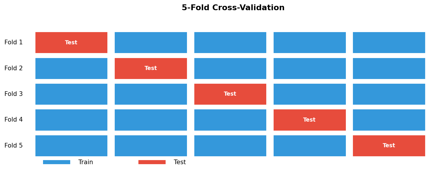
  • Recipe: split data into \(k\) equal folds. For \(i=1,\ldots,k\): train on all folds except \(i\); test on fold \(i\). Report \(\overline{\text{MSE}} \pm \text{std}(\text{MSE})\).
  • Every data point contributes to both training and testing — no waste.
  • The std tells you how stable the estimate is across splits.
  • Defaults: \(k=5\) for compute-bound situations; \(k=10\) for moderate datasets (\(N \sim 10^3\)); \(k=N\) (LOOCV) for very small datasets (\(N < 30\), common in materials science).
  • Cost: \(k\) trainings — skip for slow deep models; use repeated holdout with multiple seeds instead.

Data leakage — the silent score inflator

  • Definition: information from the test set influences the training process — directly or indirectly. The reported performance is then optimistic by an unknown amount.
  • Symptoms:
    • Cross-validation score far above performance on a new specimen or lab.
    • Even a simple model matches a deep network — both are exploiting the leak.
    • Performance drops sharply when data is collected from a different sample batch.
  • Root cause: not a bug — a discipline failure. Three main patterns:
    1. Pre-processing leakage — scaling/PCA fitted on all data before splitting.
    2. Temporal leakage — using future measurements to predict past ones.
    3. Group / spatial leakage — same physical specimen in both train and test.

The EM leakage trap: crops from one specimen

Random crop split (left, \(R^2 = 0.936\), dishonest) vs. 3-fold specimen-group split (right, mean \(R^2 = 0.169\), honest). Same synthetic dataset; the gap of 0.77 is pure leakage.
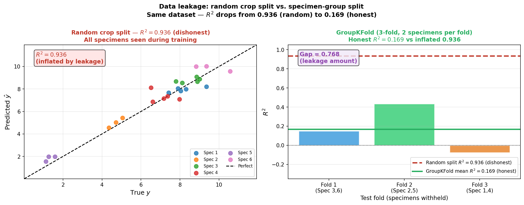
  • The scenario: 6 EM specimens, 20 crops each — 120 training examples. A per-specimen property (e.g., composition, lattice parameter, stoichiometry) is the target \(y\).
  • Random crop split (\(R^2 = 0.936\)): crops from Specimen 3 land in both train and test. The model learns “Specimen 3 looks like this” and predicts well on test crops — but it has memorised a specimen, not the property.
  • 3-fold specimen-group split (mean \(R^2 = 0.169\)): entire specimen pairs are in test only. The model must generalise across specimen identities — the honest evaluation.

The cure: specimen-level group splitting

  • Assign a group label (specimen_id) to every data point.

  • GroupKFold: the entire specimen stays in either train or test — never split across folds.

    from sklearn.model_selection import GroupKFold
    gkf = GroupKFold(n_splits=5)
    for tr, te in gkf.split(X, y, groups=specimen_id):
        model.fit(X[tr], y[tr])
        score = model.score(X[te], y[te])
  • Materials default: if there is a specimen_id column, your default CV is GroupKFold.

  • The within-specimen correlation that random CV exploits is noise from the perspective of generalisation — ignoring it inflates your score by a predictable amount.

Spot the leak — three scenarios

For each of the three setups below, identify the leakage and the fix.

(a) You standardise all features with StandardScaler().fit_transform(X) on the full dataset, then run 5-fold cross-validation.

. . .

Pre-processing leak. The scaler saw all test-set values when computing \(\mu\) and \(\sigma\). Fix: StandardScaler().fit(X_train) inside each fold (use Pipeline).

. . .

(b) You collect 100 EBSD maps from the same 5 specimens (20 maps each). You run a random 5-fold CV and report Dice=0.91. (Dice: segmentation metric — see metrics section.) On a 6th specimen, Dice=0.51.

. . .

Group leak. Maps from the same specimen in both train and test. Fix: GroupKFold(groups=specimen_id).

(c) You record an in-situ liquid-phase TEM video (1000 frames). You randomly shuffle and split 80/20. Train \(R^2 = 0.97\), deploy \(R^2 = 0.30\).

. . .

Temporal leak. Future frames used to predict past ones. Fix: train on first 800 frames; test on last 200 (chronological split).

. . .

Pattern: every leakage scenario reduces to one sentence — test-set information influenced the training process.

Temporal leakage and pre-processing leakage

  • Temporal leakage: for time-series data (operando EM, in-situ growth), randomly splitting scrambles time order. The model can use “future” frames to predict “past” ones — impossible in deployment. Fix: always split chronologically — train on \(t < t_1\), test on \(t > t_1\).

  • Pre-processing leakage: fitting a StandardScaler on all data (train + test) before splitting. Test-set statistics leak into the scaler. Fix:

    X_tr, X_te, y_tr, y_te = train_test_split(X, y)
    scaler = StandardScaler().fit(X_tr)   # fit on train only
    X_tr = scaler.transform(X_tr)
    X_te = scaler.transform(X_te)         # apply frozen scaler to test
  • sklearn.pipeline.Pipeline does the right thing automatically inside CV.

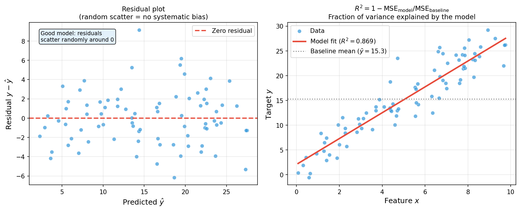
Regression metrics: MAE, RMSE, \(R^2\)

Left: residual plot with conventional \(y - \hat{y}\) on the vertical axis (random scatter around zero = good model). Right: \(R^2\) — the fraction of variance in \(y\) explained by the model.
  • \(\mathrm{MAE} = \frac{1}{n}\sum|y_i - \hat{y}_i|\) — in the same units as \(y\); robust to outliers.
  • \(\mathrm{RMSE} = \sqrt{\tfrac{1}{n}\sum(y_i - \hat{y}_i)^2}\) — in the same units as \(y\); penalises large errors more.
  • \(R^2 = 1 - \mathrm{MSE}_\text{model}/\mathrm{MSE}_\text{baseline}\) — fraction of variance explained; scale-free. \(R^2 = 1\): perfect. \(R^2 = 0\): no better than predicting \(\bar{y}\). \(R^2 < 0\): worse than baseline.
  • Always report \(R^2\) on held-out data, not training data.

Choosing the right metric — a decision tree

  • Is it a regression task? (continuous target, e.g. composition, temperature, d-spacing)
    • → Report RMSE (interpretable in physical units) and \(R^2\) (scale-free, comparable).
    • → Also plot residuals — look for systematic trends.
  • Is it a classification task? (discrete labels, e.g. defect/no defect, phase A/B/C)
    • Check class balance: are classes roughly equal? → accuracy OK.
    • Large imbalance (>5:1)? → precision, recall, F1. Never use accuracy alone.
  • Is it a segmentation task? (pixel-level mask, e.g. grain boundaries, dislocations)
    • → Report IoU or Dice (both range [0,1]).
    • Also check: precision = no false alarms, recall = no misses.
  • Key principle: the metric should match what you actually care about in the physics.

Confusion matrix — the foundation of classification metrics

For a binary defect-detection task:

Predicted: no defect Predicted: defect
True: no defect TN FP (false alarm)
True: defect FN (missed!) TP

\[\text{Accuracy} = \frac{\text{TP}+\text{TN}}{\text{TP}+\text{TN}+\text{FP}+\text{FN}}\]

  • Imbalanced classes are the norm in EM: 98% background, 2% defects. A model that always predicts “no defect” scores 98% accuracy — and misses every defect.
  • Asymmetric costs: missing a defect (FN) → unsafe part ships; calling a good part bad (FP) → unnecessary scrap. Accuracy hides this asymmetry entirely.
  • Fix: use precision and recall (next slide) — they separate the two error types.
  • For multi-class: the confusion matrix is \(K \times K\); off-diagonal entries are misclassifications.

Classification and segmentation metrics

IoU and Dice for segmentation: good overlap, over-prediction (high recall, low precision), under-prediction (high precision, low recall).
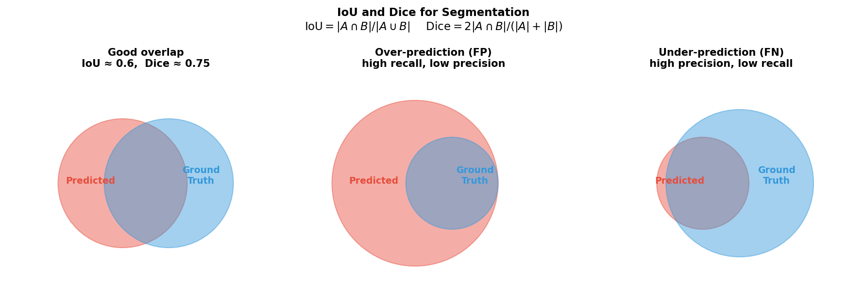
  • Precision = TP / (TP + FP) — of what I called positive, how much was correct?
  • Recall = TP / (TP + FN) — of what was truly positive, how much did I find?
  • F1 = Dice = \(2 \cdot P \cdot R / (P + R)\) — harmonic mean; penalises lopsided precision/recall.
  • IoU (Jaccard) = \(|A \cap B| / |A \cup B|\) — standard for object detection and segmentation.
  • Rule: defect detection → maximise recall. Particle picking → balance via F1/Dice.
  • \(\text{Dice} = 2\,\text{IoU}/(1 + \text{IoU})\); IoU is always ≤ Dice for the same prediction.

The full picture — an honest EM ML recipe

  1. Collect data: note the specimen structure; record specimen_id for every measurement.
  2. Inspect: histogram targets, check for duplicates; plot \(X\) vs \(y\) per specimen — if specimens cluster separately, group leakage is a risk.
  3. Split: if specimen_id exists → GroupKFold; if time-series → chronological split; otherwise 5-fold KFold.
  4. Pipeline: StandardScaler + model inside Pipeline — scaler fitted on train folds only.
  5. Fit: choose loss (MSE/MAE/Huber) based on noise model; choose optimiser (Adam default); track train and val loss per epoch.
  6. Report: test \(R^2\) or test Dice/IoU on the held-out fold; pair with residual plot or confusion matrix.
  7. Sanity check: is the honest group \(R^2\) close to the random \(R^2\)? Large gap → leakage.

What gradient descent alone cannot solve

  • Non-linear patterns: a linear model trained with GD still fits a line to non-linear data. The architecture limits expressivity, not the optimiser.
  • Bad local minima: for non-convex losses (any neural network), GD finds a minimum — not necessarily the best one. Momentum, random restarts, and SGD noise help.
  • Overfitting: minimising training loss does not guarantee good test performance. Cross-validation and regularisation are essential — GD alone cannot tell you if you have overfit.
  • Data leakage: a perfectly converged model on a leaked dataset still reports an inflated score. The optimiser cannot fix a broken validation setup.
  • Scale and ill-conditioning: ill-scaled features make GD slow regardless of the optimiser choice. Standardise inputs.

Looking ahead — Week 5

  • Topic: “Neural networks from first principles”
  • The linear predictor \(\hat{y} = \mathbf{w}^T\mathbf{x}\) is extended by stacking: outputs of one linear layer become inputs to the next, separated by non-linear activations (ReLU, sigmoid).
  • Gradient descent and Adam carry over unchanged — we just apply them to a deeper function.
  • Backpropagation is the chain rule applied to the composed function: it computes \(\nabla_\mathbf{w} \hat{R}\) efficiently without any new mathematics.
  • Prerequisite: today’s notebook — understand what an honest \(R^2\) means and why specimen-level splitting changes it.

Self-study this week

  • Notebook: notebooks/week04_leakage_demo.ipynb — “Data leakage in EM: crop-level vs. specimen-level splitting.”
    • Generate synthetic EM specimens (6 specimens, 20 correlated crops each).
    • Fit a linear regressor using (a) random crop split and (b) GroupKFold on specimen ID.
    • Confirm that the random-split \(R^2\) is inflated and the grouped \(R^2\) is lower but honest.
    • Exercise: implement the grouped split yourself and assert that grouped \(R^2 <\) random-split \(R^2\).
  • Open in Colab: no local installation; first cell installs all dependencies.
  • Goal: internalise the crop-vs-specimen distinction before Week 5.
  • Must-know review: _shared/exam_mustknow.md — Week 4 statements are now filled.

Continue

References

Pattern recognition and machine learning, Christopher M. Bishop.