Data Science for Electron Microscopy
Week 6: Neural networks & backpropagation

Prof. Dr. Philipp Pelz

FAU Erlangen-Nürnberg

Institute of Micro- and Nanostructure Research

Recap: where we left off

• Week 5: image → segmentation → regionprops / local-environment descriptors → trees, RF and GBM, validated with GroupKFold by image.
• Baseline ladder: mean → linear/Ridge → RF/GBM → neural network. Each rung must beat the one below on the same honest split.
• Week 4: training = minimising a loss, \(\theta_{t+1} = \theta_t - \eta\,\nabla_\theta\hat{R}(\theta_t)\).
• Today’s question: what if the feature map \(\boldsymbol\phi(\mathbf{x};\theta)\) itself is learned end-to-end by gradient descent — and how do we get its gradients?

• Open by asking: in the Week 5 notebook, which descriptors did the random forest rank highest for the vacancy classifier? Use the answer as the bridge: “Last week you designed the features and the trees combined them. Today the network designs the features itself.”
• The one point to land: neural networks are not a different paradigm. They live entirely inside the ERM framework from Week 4 — same loss, same gradient descent update. What changes is the model family: we replace a fixed feature map + linear/tree model by a composition of learnable nonlinear maps.
• Baseline ladder: say explicitly that every NN result in this course (notebook, miniproject) is reported next to the RF/GBM number from Week 5 on the same GroupKFold split. If the NN does not beat it, you report that honestly and use the simpler model.
• Misconception to preempt: “neural networks are magical and hard to understand.” A single neuron is a dot product plus an activation. An MLP is a chain of those. Backprop is the chain rule, organised. Today we build all three by hand.
• Pacing note: this recap slide is a bridge, not a lecture — 2 minutes maximum.
• Transition: “Here is the map for today.”

Road map and learning outcomes

Road map (≈90 min)

1. Hand-crafted vs learned features (Hall–Petch)
2. Perceptron, XOR, the dense layer
3. Activations, softmax & cross-entropy, vanishing gradients
4. Autograd & backprop — worked 2-layer example, gradient check
5. Initialisation (Xavier/He) & normalisation (batch/layer/group)
6. Diagnostics: loss curves, LR finder, overfit-one-batch
7. Regularisation, baseline ladder, when not to use a NN

After today you can …

• write an MLP forward pass in matrix form and count its parameters;
• match output activation and loss;
• backprop by hand through a small network and verify with autograd + finite differences;
• explain vanishing/exploding gradients and the fixes (ReLU, init, normalisation);
• diagnose a run from its loss curves;
• justify a NN only if it beats RF/GBM on the same split.

Self-study: notebooks/week06_tiny_mlp.ipynb

• Orientation only — 2 minutes. Point at the two anchors: (1) the Hall–Petch comparison at the start and (2) the worked backprop example in block 4. Those are the two things students should be able to reproduce on paper at the exam — expect a small hand-backprop question (2-layer ReLU network, a handful of numbers).
• Outcomes on init / normalisation / diagnostics are the practical survival skills: most “my network does not learn” questions in the miniproject are answered by init, normalisation, learning rate, or a bug that the overfit-one-batch test would have caught.
• Misconception to preempt: “if the training loss goes down, everything is fine.” Validation curves and the baseline ladder decide.
• Forward link: Week 7 adds spatial structure (convolution) on top of today’s MLP skeleton; everything about backprop, init, normalisation and diagnostics carries over unchanged.
• Timing plan (90 min, lecture path):
  • 0–5: recap + road map (2 slides)
  • 5–9: hand-crafted vs learned features (Hall–Petch, fixed → learned) (2)
  • 9–19: perceptron, XOR, dense layer, why nonlinearity (4)
  • 19–27: activations, softmax + CE, vanishing gradients, training = ERM (4)
  • 27–53: backprop block — why backprop, chain rule, graph, forward vs reverse, worked example 1–3, delta recursion, PyTorch, gradient check (10) — the core, do not rush
  • 53–65: exploding gradients, initialisation (2 slides + simulation), normalisation (5)
  • 65–74: loss curves, LR finder, sanity checks, overfitting/dropout (4)
  • 74–80: baseline ladder, when not to use a NN, training recipe (3)
  • 80–85: notebook, summary, must-know, next week (4)
  • 85–90: slack / questions (the slide-time estimate is ≈67 min; the rest is budgeted for board work: worked example, variance argument, loss-curve quiz)
• Backup slides after the “Continue” slide (information bottleneck, ADALINE, hierarchical features, historical activations, early-stopping curve, complete hardness example) are for questions only.
• Transition: “Start with the question every EM materials scientist faces: how do you turn a microstructure measurement into a number that predicts a property?”

Hall–Petch: hand-crafted vs learned features

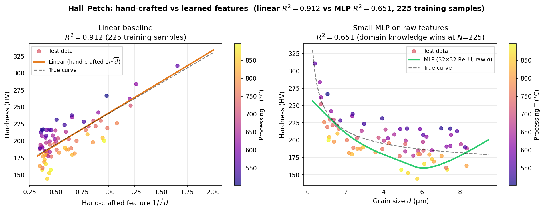
Left: linear regression on the hand-crafted \(1/\sqrt{d}\) feature achieves \(R^2\approx0.91\) (225 training samples). Right: a small MLP on raw grain size \(d\) only reaches \(R^2\approx0.65\) — with limited data, domain knowledge still wins over learned features.

• \(H = H_0 + k\,d^{-1/2}\): the engineer supplies \(\phi(d) = d^{-1/2}\). With many interacting inputs (composition, \(T_\text{proc}\), cooling rate) the right \(\phi\) is unknown — a network learns it from data.

• The Hall–Petch story is the perfect opener: the hand-crafted feature is known and correct (so we can establish the baseline), and adding more features makes hand-engineering intractable.
• Walk through the two panels. Left: “We told the model the functional form. Result: \(R^2 \approx 0.91\) with 225 training points.” Right: “We gave the model raw \(d\) and let it find the transformation. The small MLP reaches \(R^2 \approx 0.65\) — it is learning, but domain knowledge still wins at this sample size.”
• The one point to land: feature engineering is the hidden work in classical ML. Networks move that work from the human to the optimiser — trading expert effort for data. Neither is always better.
• Misconception to preempt: “a deep network always beats hand-crafted features.” It does not — especially when \(N\) is small. When the domain knowledge is correct, embed it. Use learned features when the physics is unclear or multi-factorial.
• EM anchor: EELS near-edge fine structure, EBSD texture, EDS compositional interactions — cases where the correct feature transformation is not analytically known. That is where networks earn their place.
• Optional (backup slide): the information-bottleneck argument — a 10⁶-pixel micrograph collapsed to one ASTM grain-size number Sandfeld, Stefan et al., (2024).
• Transition: “Let’s state the change precisely.”

From fixed to learned feature maps

• Fixed basis (up to Week 5): \(\hat{y} = \sum_j w_j\,\phi_j(\mathbf{x})\) — Fourier, polynomial, \(1/\sqrt{d}\), regionprops; only \(w_j\) is learned.
• Neural network: \(\phi_j(\mathbf{x};\theta)\) is learnable. The architecture decides which features are easy to learn; training finds them.

Hand-crafted features encode what the engineer knows. Learned features encode what the data contains.

• Connect to the basis-function material students may know: Fourier series, polynomial regression. All of these are fixed-basis models. Neural networks generalise this by making the basis itself learnable.
• The one point to land: the transition from fixed to learned features is the single biggest conceptual leap in modern ML. Everything else — architecture choices, training tricks — is an engineering consequence.
• Misconception to preempt: “learned features are always better.” They require more data, more compute, and more validation discipline. In data-sparse EM regimes (N < 100 specimens), domain-knowledge features are often superior.
• EM anchor: a physicist fitting EELS edges uses a hand-crafted basis (atomic cross-sections). A network would learn basis functions from thousands of labelled spectra.
• Transition: “Build from the ground up. The atom of every neural network is a single neuron.”

The perceptron: one neuron, one hyperplane

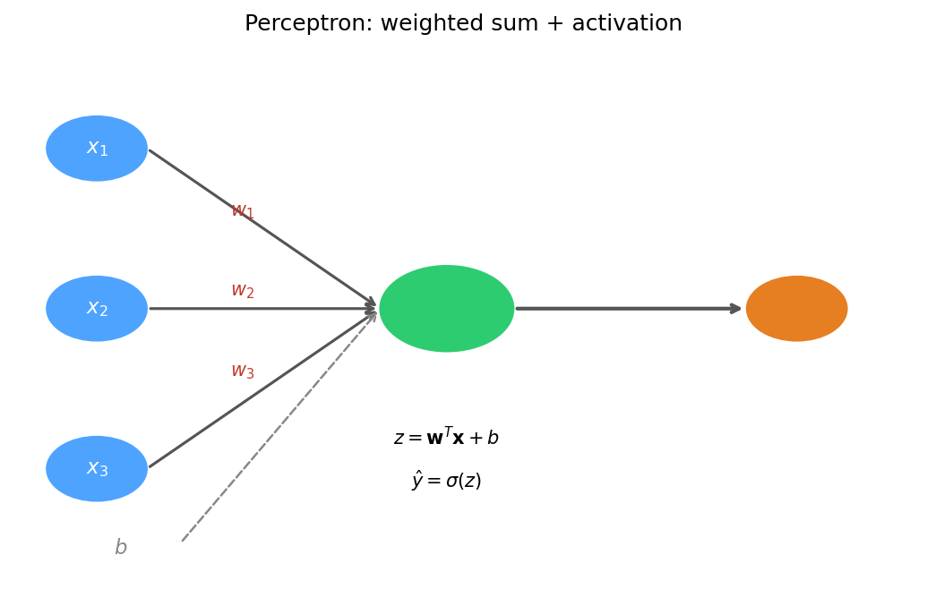
A single perceptron: inputs \(x_i\) weighted by \(w_i\), bias \(b\) added, sum passed through an activation \(\sigma\).

• \(a = \sigma(\mathbf{w}^\top\mathbf{x} + b)\)
• Boundary \(z = \mathbf{w}^\top\mathbf{x} + b = 0\) is a hyperplane (a line in 2-D).
• Trained with gradient descent on a loss, this is Week 4’s linear / logistic regression.
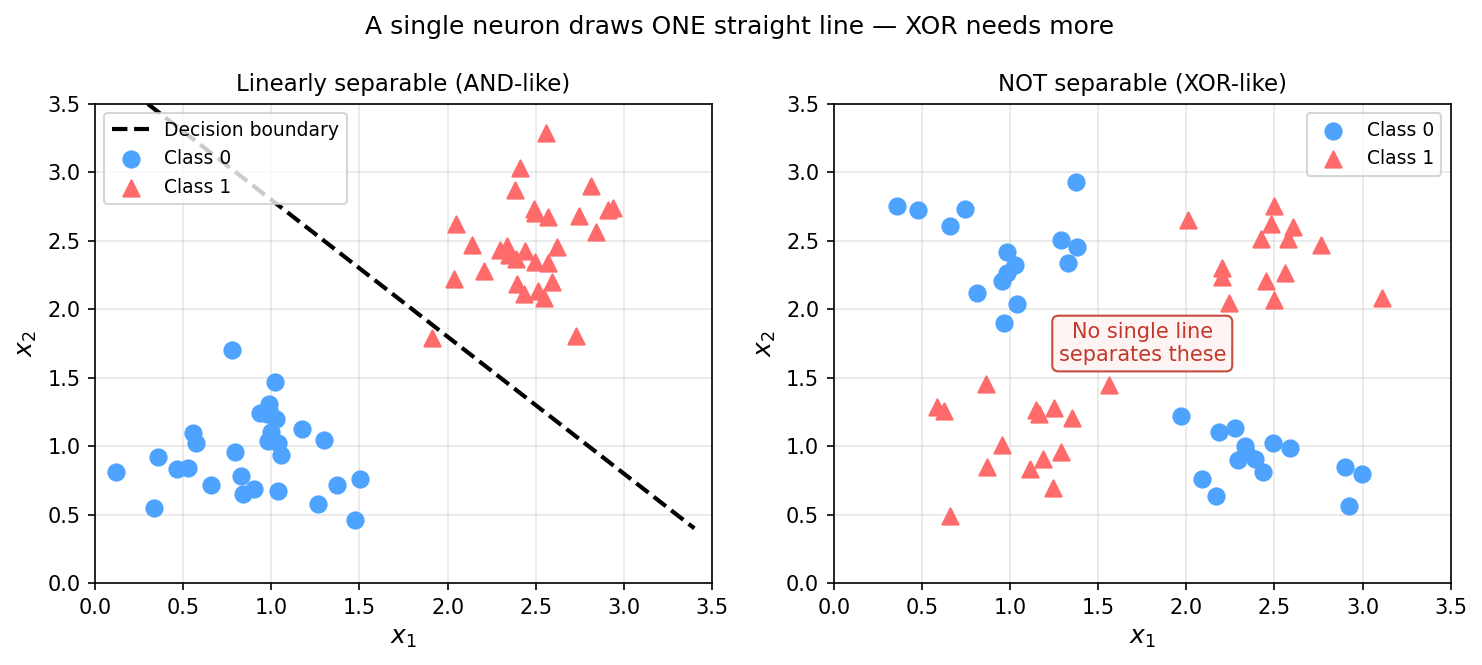
• One neuron = one straight line. It cannot curve.

• Draw this on the board while talking through it: weighted sum, bias as the threshold, then a nonlinear activation. Then draw two axes \(x_1, x_2\), two classes, and the boundary line \(w_1x_1 + w_2x_2 + b = 0\).
• Keep this short: students saw linear models in Week 4. The neuron with identity activation + MSE is linear regression (historically ADALINE, 1960 — backup slide); with sigmoid + BCE it is logistic regression.
• Misconception to preempt: “the bias is optional.” Without bias all boundaries pass through the origin.
• Misconception to preempt: “the perceptron always converges.” The Perceptron Convergence Theorem only holds for linearly separable data.
• EM anchor: classify “pore” vs “grain” pixels in a BSE image from two features (contrast, local std). If the classes overlap in a curved way, no single threshold line works.
• Transition: “Where exactly does one line fail?”

XOR: why a hidden layer is needed

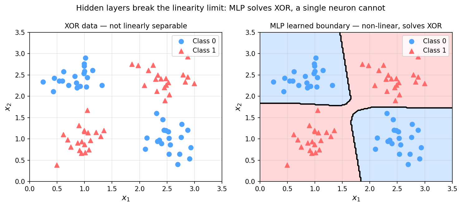
AND-like data: one line separates the classes. XOR: no single line can.

An MLP with hidden layers learns a curved boundary that classifies all four XOR quadrants.

• The hidden layer warps the input space into learned features where a final linear boundary suffices.

• Left figure first: ask the room “Can you draw a straight line that puts blue dots on one side and red triangles on the other?” Nobody can — that is a mathematical impossibility for a linear classifier, not a training failure.
• Right figure: the curved boundary is not drawn by a single neuron; it emerges from combining linear thresholds separated by nonlinear activations. A 2→2→1 network already suffices Goodfellow, Ian et al., (2016).
• The one point to land: hidden layers are feature engineers that adapt to the data; the last layer is just a linear classifier on those features. True for every MLP and every CNN.
• Misconception to preempt: “XOR is a toy problem.” Curved or multi-connected decision boundaries are everywhere in microstructure classification — three-phase alloys, EBSD orientation classes, defect vs clean regions in HAADF.
• Misconception to preempt: “more neurons always help.” More capacity also means more overfitting risk; validation decides.
• Transition: “Now write the layer down as a matrix multiply.”

The dense layer: matrix view and parameter count

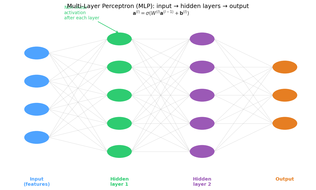
An MLP: hidden layers learn internal representations; the output layer is a linear map on them.

\[\mathbf{z} = W\mathbf{x} + \mathbf{b}, \qquad \mathbf{a} = \sigma(\mathbf{z})\]

• \(W \in \mathbb{R}^{M \times D}\), \(\mathbf{b} \in \mathbb{R}^M\). Batch: \(A = \sigma(WX + \mathbf{b})\), bias broadcasts.
• Parameters: \(M(D+1)\). Example: \(D=20\), \(M=64\) → 1,344.

• Walk the diagram left to right: input layer (no computation), hidden layers (dot product + bias + activation for every neuron), output layer (final linear combination).
• Name shapes slowly: x is D by 1, W is M by D, output is M by 1. D=20, M=64 gives 1280 weights + 64 biases = 1344.
• The one point to land: dense means every input can affect every output. Powerful but expensive — for images this leads to billions of parameters (which motivates CNNs in Week 7).
• Misconception to preempt: “the batch size N affects the number of parameters.” It does not.
• EM anchor: 20 composition + process features, 20 → 64 → 64 → 1 has 1344 + 4160 + 65 ≈ 5569 parameters. With N=300 training samples, regularisation is needed.
• Transition: “Why do we need the \(\sigma\) at all?”

Why non-linearity is non-negotiable

• Two purely linear layers: \[W^{(2)}\bigl(W^{(1)}\mathbf{x}+\mathbf{b}^{(1)}\bigr)+\mathbf{b}^{(2)} = \underbrace{(W^{(2)}W^{(1)})}_{\tilde{W}}\mathbf{x}+\tilde{\mathbf{b}}\]
• Any depth of linear layers = one affine map. Depth without nonlinearity is no depth at all — and XOR stays unsolvable.

• Write \(W^{(2)}W^{(1)} = \tilde{W}\) on the board. “No matter how many weights we have in two layers, they compose into a single weight matrix.”
• The one point to land: each nonlinearity creates a kink/threshold that lets the next layer represent structure that was not representable before.
• Misconception to preempt: “I can stack 50 linear layers and get 50× better performance.” The collapse algebra kills this — the most common conceptual error for newcomers.
• Universal approximation: one wide enough hidden layer with a nonlinearity can approximate any continuous function; the limits of that promise come near the end. Hierarchical-feature intuition: backup slide.
• Transition: “Which nonlinearity? A quick survey.”

Activation functions: what to use where

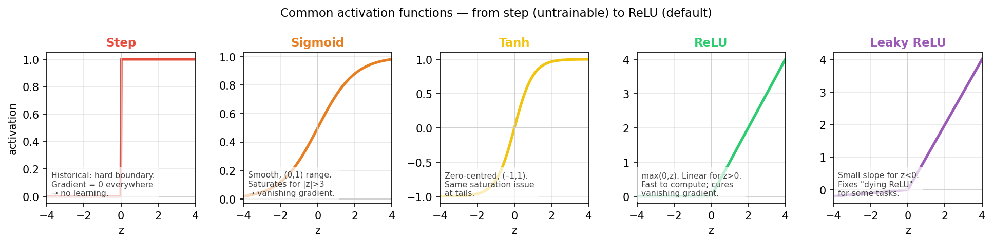
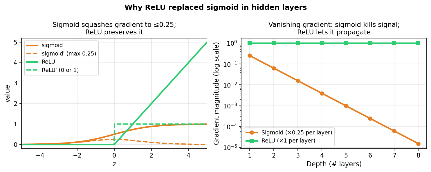
Step, sigmoid, tanh, ReLU, Leaky ReLU. ReLU preserves the gradient for positive inputs; sigmoid and tanh saturate.

• Hidden layers: ReLU \(\max(0,z)\) — gradient exactly 1 for \(z>0\), cheap. Step: zero gradient, untrainable. Sigmoid \(\sigma' \le 0.25\) and tanh saturate for \(|z| \gtrsim 3\) — used at outputs, not inside.

• Walk left to right. Step: the McCulloch–Pitts neuron — gradient zero everywhere, impossible to train by gradient descent. Sigmoid: smooth, \(\sigma' = \sigma(1-\sigma) \le 0.25\), saturates. Tanh: zero-centred sigmoid, max gradient 1 at 0, same saturation. ReLU: identity above zero, zero below — does not saturate for positive inputs, the default since AlexNet (2012). Leaky ReLU: small negative slope against dying neurons.
• The one point to land: hidden layers use ReLU; output uses identity (regression), sigmoid (binary) or softmax (multi-class).
• Misconception to preempt: “sigmoid is a good default for hidden layers.” It was in 1990; its saturation is what stalled deep networks until ~2012.
• Details on step/sigmoid/tanh history: backup slide.
• Transition: “The output layer deserves one more slide.”

Output layer: softmax and matched losses

• \(K\) classes: \(\hat{p}_k = e^{z_k} / \sum_j e^{z_j}\) — a probability vector. Cross-entropy \(\mathcal{L} = -\sum_k y_k \log \hat{p}_k\); the output gradient is simply \(\hat{\mathbf{p}} - \mathbf{y}\).

Task	Output activation	Loss
Regression	identity	MSE or MAE
Binary classification	sigmoid	binary cross-entropy
Multi-class	softmax	categorical cross-entropy

• Softmax generalises sigmoid to \(K\) classes: outputs positive and summing to 1. Sigmoid per class would give independent outputs that can sum to more than 1.
• The one point to land: output activation and loss must be matched. Softmax + CE gives the beautifully simple gradient \(\hat p - y\) — the same “prediction minus target” as linear regression with MSE. We will see it again in the delta recursion.
• Misconception to preempt: “I can use MSE with a softmax output.” Possible, but the gradient landscape is poor.
• EM anchor: phase classification with \(K=4\) phases (ferrite, austenite, martensite, bainite): 4 output neurons + softmax, categorical CE, prediction = argmax.
• Transition: “Why did sigmoid disappear from hidden layers? Vanishing gradients.”

Vanishing gradients: why ReLU won

Left: sigmoid gradient ≤ 0.25, ReLU gradient = 1 for \(z>0\). Right: at depth 8 sigmoid gradients have shrunk by four orders of magnitude; ReLU gradients stay at full strength.

• The chain rule multiplies one \(\sigma'\) per layer.
• Sigmoid: \(\le 0.25^8 \approx 2\times10^{-4}\) after 8 layers → early layers barely learn Goodfellow, Ian et al., (2016).
• ReLU: factor 1 for active units → depth becomes trainable.

• Write on the board: \(\partial \mathcal{L}/\partial W^{(1)} = \delta^{(L)} \cdot \sigma'(z^{(L-1)}) \cdot W^{(L)} \cdots \sigma'(z^{(1)}) \cdot W^{(2)}\). “Each factor \(\sigma'\) is at most 0.25.”
• Read the right panel: at depth 8, sigmoid gradient \(10^{-4}\), ReLU 1 — four orders of magnitude.
• The one point to land: vanishing gradients are a structural consequence of activation derivatives below 1, not a precision issue. Historically this is why networks beyond ~5 layers were almost untrainable before 2012.
• Misconception to preempt: “a smaller learning rate fixes vanishing gradients.” It makes things worse. The fixes are ReLU, init, normalisation and residual connections (Week 7).
• Transition: “We have the architecture. How does it learn? Same as Week 4.”

Training a network: the same ERM loop

\[\hat{R}(\theta) = \frac{1}{N}\sum_{i=1}^{N} \mathcal{L}\!\bigl(f_\theta(\mathbf{x}_i),\, y_i\bigr), \qquad \theta \leftarrow \theta - \eta\,\nabla_\theta \hat{R}\]

• \(\theta\) = all weights and biases of all layers; \(f_\theta\) is a composition of nonlinear maps; the loss surface is non-convex.
• SGD / Adam as before — Adam at \(\eta = 10^{-3}\) is the usual start.
• The only new problem: computing \(\nabla_\theta\hat{R}\) for \(10^4\)–\(10^9\) parameters.

• Emphasise continuity with Week 4: “The formula is identical. The only change is that \(f_\theta\) is a few matrix multiplications and activations instead of one dot product.”
• Misconception to preempt: “we must find the global minimum.” Gradient descent finds a local minimum; well-initialised networks find ones that generalise well. Plateaus and saddle points are the practical problem.
• EM anchor: calling optimizer.step() in PyTorch executes this update once per mini-batch; for a typical miniproject dataset the loop runs thousands of times.
• Transition: “So the challenge is the gradient. How do we get it cheaply?”

Why we need backpropagation

Method	Passes needed	Cost for \(W\) params	Exact?
Finite differences	\(W+1\) forward	\(O(W^2)\)	no (\(\epsilon\) error)
Symbolic	—	expression swell	yes
Backprop (reverse AD)	1 forward + 1 backward	\(O(W)\)	yes

• For \(W = 10^6\): backprop is \(\sim10^6\times\) cheaper Rumelhart, David E. et al., (1986); Baydin, Atılım Güneş et al., (2018); Bishop, Christopher M., (2006).
• Finite differences keep one job: checking gradients (end of this block).

• Make the cost argument concrete: \(10^6\) weights, forward pass 1 ms. Finite differences: \(10^6\) forward passes = 17 minutes per gradient step. Backprop: ~2–3 ms. That factor is why deep learning exists.
• Finite differences formula for reference: \(\partial\hat R/\partial\theta_j \approx [\hat R(\theta+\epsilon\mathbf{e}_j) - \hat R(\theta)]/\epsilon\) — one extra forward pass per parameter, each of cost \(O(W)\), plus round-off error.
• Symbolic differentiation gives exact formulas but the written-out derivative of a 10-layer net is enormous.
• The one point to land: backprop is not an approximation and not a symbolic formula — it evaluates the chain rule on numbers, in the right order, reusing intermediate results.
• Misconception to preempt: “autodiff is numerical differentiation.” There is no \(\epsilon\) and no truncation error.
• EM anchor: gradient-based ptychography (Week 13): millions of object pixels, one scalar loss — exactly the case where reverse mode wins.
• Transition: “Everything rests on the chain rule.”

Chain rule: the only calculus you need

• Univariate: \(y = f(g(x)) \Rightarrow dy/dx = f'(g(x))\,g'(x)\).
• Multivariate: \(L\) depends on \(x\) through \(u_1,\dots,u_k\): \[\frac{\partial L}{\partial x} = \sum_{i=1}^{k} \frac{\partial L}{\partial u_i}\,\frac{\partial u_i}{\partial x}\] → multiply along each path, sum over paths.
• Vector form: Jacobians compose by matrix multiplication.

• Concrete example: \(y = \sin(x^2)\), \(dy/dx = \cos(x^2)\cdot 2x\).
• The one point to land: “multiply along paths, sum over paths.” A hidden unit feeds many units of the next layer — the sum over paths is exactly the \(\sum_m w_{mk}\delta_m\) of the delta recursion.
• Misconception to preempt: “I have to form the huge Jacobian.” Never — only vector–Jacobian products \(\mathbf{v}^T J\), which are cheap. That is what backward() computes.
• Transition: “Now put these rules on a graph.”

Autograd: backprop on the computational graph

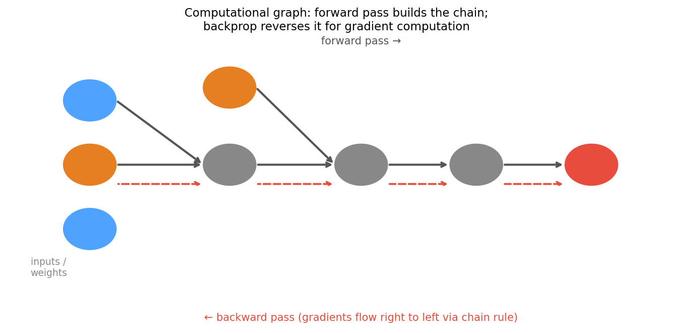
Computational graph for one neuron: forward pass (black, left to right) computes the loss; backward pass (red dashed, right to left) propagates gradients via the chain rule at each node.

• Forward: evaluate nodes left to right; store intermediates.
• Backward: right to left, multiply the incoming gradient by each node’s local derivative.
• PyTorch/JAX build the graph as your code runs: loss.backward() fills .grad.

• Walk through the graph. Forward: \(x_1 \cdot w_1\), add \(b\) → \(z\), \(\sigma\) → \(a\), loss \(\mathcal{L}\). Backward: gradient 1 at the loss; multiply by \(\sigma'(z)\) at the activation; the add node passes through; at the multiply node, gradient w.r.t. \(w_1\) = chain product × input \(x_1\).
• The one point to land: each node has a simple local derivative; the full gradient is the product of local derivatives from the output back to the weight. Exact, efficient, automatic.
• Misconception to preempt: “backprop is only for neural networks.” It is reverse-mode AD — it applies to any differentiable computation, including physics forward models (Weeks 12–13).
• Extra reading: the SS25 autograd notebook (data_science_for_em/01_intro/01_autograd.qmd) and the MFML Unit 4 backprop self-study.
• Transition: “Why right to left, and not left to right?”

Forward mode vs reverse mode

• Forward mode: one pass per input — efficient when #inputs ≪ #outputs.
• Reverse mode: one pass per output — efficient when #outputs ≪ #inputs.
• Training maps \(10^4\)–\(10^9\) parameters → one scalar loss ⇒ reverse mode = backpropagation.
• Price: store all \(\mathbf{z}^{(\ell)}, \mathbf{a}^{(\ell)}\) — memory, not compute, is the limit for large EM images.

• Analogy: forward mode asks “if I wiggle this one input, how do all outputs move?”; reverse mode asks “for this one output, how much is each input to blame?”. Training needs blame assignment for one loss.
• The one point to land: backprop’s cost is about 2–3× a forward pass, independent of the number of parameters; memory is proportional to the stored activations.
• Misconception to preempt: “GPU out-of-memory means too many parameters.” Usually it is the stored activations (batch × spatial size × channels). For 4k × 4k EM images activations dominate — hence patches/tiles and gradient checkpointing.
• Transition: “Enough theory — let’s do one by hand.”

Worked example (1/3): the network and the forward pass

Network: 1 input → 2 ReLU hidden units → 1 linear output, squared loss.

\[ \begin{aligned} \mathbf{z}^{(1)} &= \mathbf{W}^{(1)}x + \mathbf{b}^{(1)}, &\quad \mathbf{a}^{(1)} &= \mathrm{ReLU}(\mathbf{z}^{(1)})\\ \hat{y} &= \mathbf{w}^{(2)\top}\mathbf{a}^{(1)} + b^{(2)}, &\quad L &= \tfrac12(\hat{y}-y)^2 \end{aligned} \]

Numbers: \(x = 1,\; y = 0.5\), \(\mathbf{W}^{(1)} = \begin{pmatrix}2\\-1\end{pmatrix}\), \(\mathbf{b}^{(1)} = \begin{pmatrix}-0.5\\0.5\end{pmatrix}\), \(\mathbf{w}^{(2)} = \begin{pmatrix}1\\2\end{pmatrix}\), \(b^{(2)} = 0\).

• \(\mathbf{z}^{(1)} = (2\cdot1-0.5,\; -1\cdot1+0.5) = (1.5,\,-0.5)\)
• \(\mathbf{a}^{(1)} = \mathrm{ReLU}(\mathbf{z}^{(1)}) = (1.5,\; 0)\) ← unit 2 is off
• \(\hat{y} = 1\cdot1.5 + 2\cdot0 + 0 = 1.5\)
• \(L = \tfrac12(1.5-0.5)^2 = 0.5\)
• Store \(\mathbf{z}^{(1)}, \mathbf{a}^{(1)}, \hat y\) — the backward pass needs them.

• Do this on the board, live, with the class calling out numbers. It takes 3 minutes and is the most valuable 3 minutes of the lecture for the exam.
• The one point to land: the forward pass is just evaluating the formula — but we write down every intermediate value, because each one reappears in the backward pass.
• Misconception to preempt: “ReLU is not differentiable at 0, so backprop breaks.” In practice \(z=0\) exactly never happens with floating-point weights; frameworks use \(\mathrm{ReLU}'(0) = 0\). Here we deliberately chose \(z_2^{(1)} = -0.5\) to see what an inactive unit does.
• Same numbers are used in the notebook gradient-check cell — students can verify by running it.
• Transition: “Now we go backwards.”

Worked example (2/3): the backward pass

• Output: \(\delta^{(2)} = \dfrac{\partial L}{\partial \hat y} = \hat{y} - y = 1.0\)
• Output-layer parameters: \(\dfrac{\partial L}{\partial \mathbf{w}^{(2)}} = \delta^{(2)}\,\mathbf{a}^{(1)} = (1.5,\; 0)\), \(\quad\dfrac{\partial L}{\partial b^{(2)}} = \delta^{(2)} = 1.0\)
• Into the hidden layer: \(\dfrac{\partial L}{\partial \mathbf{a}^{(1)}} = \mathbf{w}^{(2)}\,\delta^{(2)} = (1.0,\; 2.0)\)
• Through ReLU: \(\boldsymbol{\delta}^{(1)} = \dfrac{\partial L}{\partial \mathbf{z}^{(1)}} = (1.0,\,2.0) \odot \mathrm{ReLU}'(\mathbf{z}^{(1)}) = (1.0,\,2.0)\odot(1,\,0) = (1.0,\; 0)\)
• Hidden-layer parameters: \(\dfrac{\partial L}{\partial \mathbf{W}^{(1)}} = \boldsymbol{\delta}^{(1)}\,x = (1.0,\; 0)\), \(\quad \dfrac{\partial L}{\partial \mathbf{b}^{(1)}} = \boldsymbol{\delta}^{(1)} = (1.0,\; 0)\)
• GD step (\(\eta = 0.1\)): \(w^{(2)}_1: 1 \to 0.85\), \(W^{(1)}_1: 2 \to 1.9\), \(b^{(1)}_1: -0.5\to-0.6\); unit 2’s incoming weights do not move this step.

• Pattern to highlight on the board: every weight gradient is “(error signal arriving at the node) × (input that the weight multiplied in the forward pass)”. That is why we stored the activations.
• The one point to land: the inactive ReLU unit blocks the gradient — \(\mathrm{ReLU}'=0\) — so its incoming weights get zero gradient for this sample. If a unit is inactive for every sample, it never recovers: a “dead ReLU”.
• Misconception to preempt: “the gradient w.r.t. \(w^{(2)}_2\) is zero because \(w^{(2)}_2\) is unimportant.” No — it is zero because the activation it multiplies is zero for this sample. Gradients are per-sample; the mini-batch average mixes many samples.
• Quick check with the class: after the GD step, recompute \(\hat y\) (\(z_1 = 1.9 - 0.6 = 1.3\), \(\hat y = 0.85 \cdot 1.3 + 0 - 0.1 = 1.005\); with \(b^{(2)} \to -0.1\)). The loss dropped from 0.5 to about 0.13 — the step worked.
• Transition: “Here is the same computation drawn on the graph.”

Worked example (3/3): the whole thing on one graph

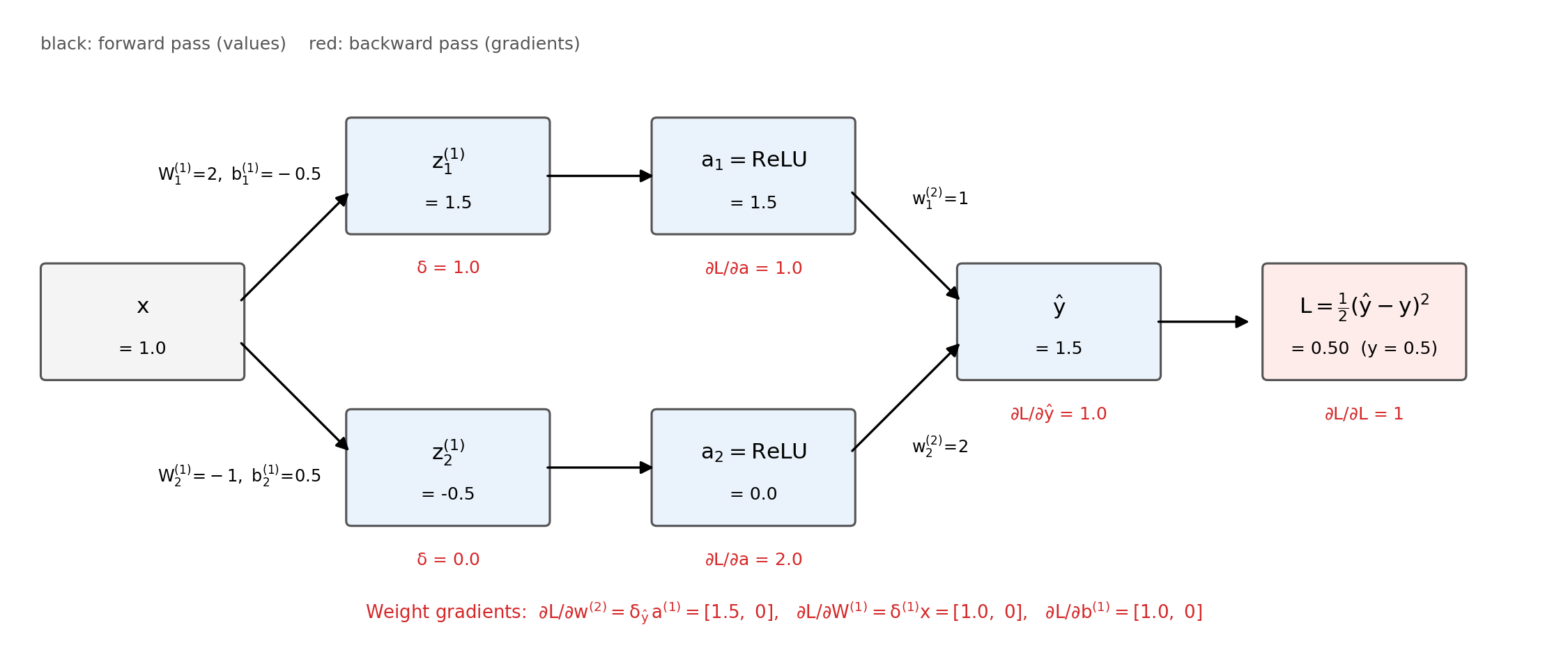
Forward values (black) and backward gradients (red) for the worked example. Each weight gradient = incoming error signal × stored forward input. The inactive ReLU unit (\(z_2^{(1)}<0\)) passes no gradient. Figure: img/make_figures.py.

• Trace the red numbers right to left with a pointer: 1 at the loss, 1.0 at \(\hat y\), split into 1.0 and 2.0 at the two activations, then the ReLU gate multiplies by 1 and 0.
• The one point to land: backprop is local. Each node only needs its own local derivative and the gradient arriving from the right. That locality is what lets frameworks implement it for arbitrary code.
• EM anchor: replace the ReLU nodes by an FFT, a probe multiplication and \(|\cdot|^2\) and this is the graph of a ptychographic forward model (Week 13). The backward pass works identically.
• Transition: “Now generalise the recipe to any depth.”

The delta recursion and the backprop algorithm

1. Forward: \(\mathbf{z}^{(\ell)} = \mathbf{W}^{(\ell)}\mathbf{a}^{(\ell-1)} + \mathbf{b}^{(\ell)}\), \(\mathbf{a}^{(\ell)} = \sigma(\mathbf{z}^{(\ell)})\); store both (\(\mathbf{a}^{(0)} = \mathbf{x}\)).
2. Output delta: \(\boldsymbol{\delta}^{(L)} = \nabla_{\mathbf{a}^{(L)}}\mathcal{L} \odot \sigma'(\mathbf{z}^{(L)})\)
3. Backward, \(\ell = L-1..1\): \[\boldsymbol{\delta}^{(\ell)} = \sigma'(\mathbf{z}^{(\ell)}) \odot \bigl(\mathbf{W}^{(\ell+1)\top}\boldsymbol{\delta}^{(\ell+1)}\bigr)\]
4. Gradients: \(\nabla_{\mathbf{W}^{(\ell)}}\mathcal{L} = \boldsymbol{\delta}^{(\ell)}\mathbf{a}^{(\ell-1)\top}\), \(\;\nabla_{\mathbf{b}^{(\ell)}}\mathcal{L} = \boldsymbol{\delta}^{(\ell)}\)

• \(\mathbf{W}^{\top}\boldsymbol\delta\) = “sum over paths”.
• \(\odot\,\sigma'\) = local gate (ReLU passes/blocks, sigmoid shrinks ≤ 0.25).
• Softmax + CE: \(\boldsymbol\delta^{(L)} = \hat{\mathbf{p}} - \mathbf{y}\).

• Map every line back to the worked example: step 2 gave \(\delta^{(2)}=1\), step 3 gave \((1,0)\), step 4 gave the weight gradients.
• The one point to land: backprop is four lines. The backward pass reuses the transposed forward weights — information flows back along the same edges.
• Misconception to preempt: “each layer needs its own derivation.” No — the recursion is identical for every layer; only \(\sigma'\) and the loss derivative change.
• Mini-batch: average the per-sample gradients; in matrix form \(\nabla_{\mathbf{W}} = \frac{1}{B}\boldsymbol{\Delta}\mathbf{A}^\top\).
• The softmax + CE result \(\hat p - y\) is the matched output/loss pair from earlier paying off.
• This slide follows MFML Unit 4 notation; students who took MFML have seen the derivation in more detail.
• Transition: “In practice you never write this yourself. Here is what PyTorch does.”

Autograd in PyTorch: the training step

# the training step of every network in this course
opt.zero_grad()              # gradients ACCUMULATE by default -> reset them
loss = loss_fn(model(xb), yb)
loss.backward()              # reverse-mode AD: fills p.grad for every parameter p
opt.step()                   # theta <- theta - eta * grad  (or Adam)

• torch.no_grad() for evaluation · model.eval() switches dropout / batch norm to inference mode.

• Minimal warm-up example (from the SS25 autograd notebook), if time: x = torch.arange(4.0, requires_grad=True); y = 2*torch.dot(x, x); y.backward(); x.grad → tensor([0., 4., 8., 12.]) = \(4\mathbf{x}\) — checkable by hand.
• The one point to land: PyTorch builds the computational graph dynamically while your Python code runs — loops, if-statements and function calls are all fine. backward() then walks that graph in reverse.
• Misconception to preempt: forgetting zero_grad(). PyTorch adds new gradients to .grad (useful for gradient accumulation over micro-batches for huge EM images) — forgetting to reset gives silently wrong updates.
• tensor.detach() cuts a value out of the graph.
• Transition: “How do you know your gradients are right when you write something custom? Check them.”

Gradient checking: trust, but verify

• Central differences per parameter: \(g_j^\text{num} = \dfrac{\mathcal{L}(\theta + \epsilon\mathbf{e}_j) - \mathcal{L}(\theta - \epsilon\mathbf{e}_j)}{2\epsilon}\), error \(O(\epsilon^2)\).
• Compare with the analytic/autograd gradient via the relative error \[r = \frac{\|\mathbf{g}^\text{auto} - \mathbf{g}^\text{num}\|}{\|\mathbf{g}^\text{auto}\| + \|\mathbf{g}^\text{num}\|}\]
• Rules of thumb (float64, \(\epsilon \approx 10^{-6}\)): \(r < 10^{-7}\) fine · \(10^{-4}\) suspicious · \(> 10^{-2}\) bug.
• Use float64, a tiny model, a few samples, and turn off dropout (randomness breaks the check). Avoid kinks: ReLU at \(z \approx 0\) can give spurious mismatches.
• Notebook: manual NumPy backprop vs loss.backward() vs finite differences on the worked example and a random 2-layer net.

• This is the practical payoff of the hand-derivation: in the notebook students implement the four-line delta recursion in NumPy and compare it to PyTorch autograd and to central differences. All three must agree to ~1e-10.
• The one point to land: gradient checking is the unit test of differentiable code. Use it whenever you write a custom loss (e.g. a Poisson NLL from Week 2) or a custom differentiable forward model.
• Misconception to preempt: “float32 is fine for the check.” With float32 and \(\epsilon = 10^{-6}\), round-off dominates and you get \(r \sim 10^{-3}\) even for correct code. Always check in float64.
• Transition: “Correct gradients can still be useless if they vanish or explode through depth.”

Exploding gradients and gradient clipping

• Backward pass = product of \(L\) factors \(\mathrm{diag}(\sigma'(\mathbf{z}^{(\ell)}))\,\mathbf{W}^{(\ell+1)\top}\).
• Factors \(< 1\) → vanish (sigmoid, tiny weights); factors \(> 1\) → explode (large weights) → loss jumps, then NaN.
• Clipping (safety net): if \(\|\nabla\| > \tau\), rescale to norm \(\tau\) — clip_grad_norm_(model.parameters(), 1.0).
• Structural fixes keep each factor ≈ 1: ReLU, initialisation, normalisation, residual connections (Week 7).

• Connect to the vanishing-gradient slide: same product, other direction. The healthy regime is a product of factors near 1.
• Clipping formula: \(\nabla_\theta\mathcal{L} \leftarrow \tau\,\nabla_\theta\mathcal{L}/\|\nabla_\theta\mathcal{L}\|\); in PyTorch torch.nn.utils.clip_grad_norm_.
• The one point to land: clipping treats the symptom (one bad step), initialisation and normalisation treat the cause (the scale of each factor).
• Misconception to preempt: “NaN loss means my data has NaNs.” Check that first — but more often the learning rate is too high or gradients exploded. Clipping + lower LR is the first fix to try.
• EM anchor: unnormalised raw detector counts (0–60 000 for a 16-bit camera) fed straight into a network are a classic cause of exploding activations in the first iteration.
• Transition: “The first structural fix costs nothing: start with weights of the right size.”

Initialisation: symmetry breaking and scale

• Zero / constant init: all hidden units compute the same output, get the same gradient → the layer behaves like one neuron forever. Always wrong (biases may start at 0).
• Scale: too small → signals shrink layer by layer; too large → explode (ReLU) or saturate (tanh).
• Xavier / Glorot Glorot, Xavier et al., (2010): \(\mathrm{Var}(w) = \dfrac{2}{D_\text{in}+D_\text{out}}\) — tanh/sigmoid.
• He / Kaiming He, Kaiming et al., (2015): \(\mathrm{Var}(w) = \dfrac{2}{D_\text{in}}\) — ReLU (a variance; std \(= \sqrt{2/D_\text{in}}\)).

• Draw why zero-init fails: “If all weights are zero, all hidden units output the same value; all gradients are identical; after the update they are still identical.”
• The one point to land: initialisation is about scale. The variance of activations (forward) and gradients (backward) should stay roughly constant from layer to layer.
• Misconception to preempt: “Adam makes initialisation irrelevant.” Adam rescales step sizes; it does not break symmetry and does not rescue activations that are already \(10^{-16}\) or \(10^{19}\) at step 0.
• Defaults: PyTorch nn.Linear uses a Kaiming-uniform variant; sklearn MLPRegressor uses Glorot-uniform. Override only deliberately (torch.nn.init.kaiming_normal_).
• Transition: “Where does the factor 2/D_in come from? Three lines of variance algebra.”

Why \(\mathrm{Var}(w) = 2/D_\text{in}\): the variance argument

• \(z = \sum_{j=1}^{D_\text{in}} w_j a_j\), independent zero-mean weights: \[\mathrm{Var}(z) = D_\text{in}\,\mathrm{Var}(w)\,\mathbb{E}[a^2]\]
• Linear/tanh: \(\mathbb{E}[a^2] \approx \mathrm{Var}(z_\text{prev})\) → \(\mathrm{Var}(w) = 1/D_\text{in}\) (Xavier averages in/out).
• ReLU zeroes half: \(\mathbb{E}[a^2] = \tfrac12\mathrm{Var}(z_\text{prev})\) → \(\mathrm{Var}(w) = 2/D_\text{in}\) (He).
• Otherwise a factor \(c^L\) after \(L\) layers: \(0.5^{20} \approx 10^{-6}\), \(2^{20} \approx 10^{6}\).

• Do this on the board; it is short. Facts used: variance of a sum of independent terms adds; \(\mathrm{Var}(wa) = \mathrm{Var}(w)\mathbb{E}[a^2]\) for zero-mean independent \(w\).
• The one point to land: the same exponential \(c^L\) that kills gradients also governs the forward activations. Getting \(c = 1\) at initialisation is the whole trick.
• Misconception to preempt: “this only matters for 100-layer networks.” Even 5–10 layers with a bad scale train slowly or not at all.
• Transition: “Here is that argument as a simulation.”

Initialisation in action: activation scale through depth

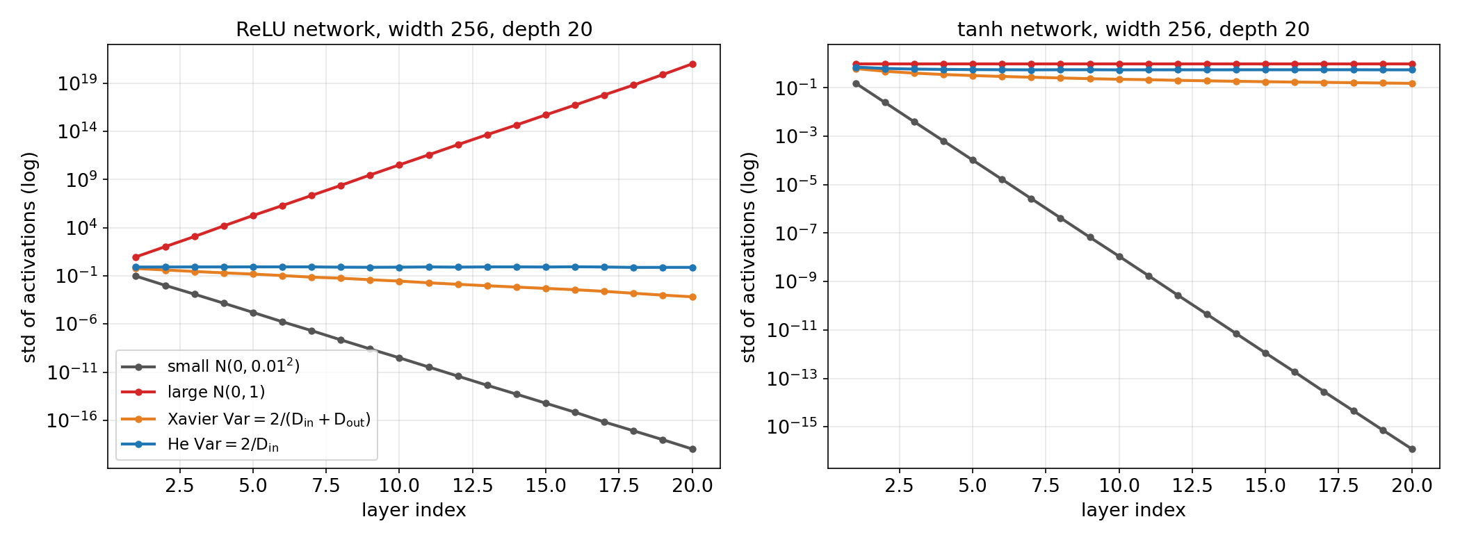
Standard deviation of activations layer by layer in a 20-layer, width-256 network fed with unit-variance input. ReLU (left): small weights → activations vanish, \(\mathcal{N}(0,1)\) → explode, Xavier → slow decay, He → constant. tanh (right): large weights saturate at ±1, small weights vanish, Xavier/He stay usable. Figure: img/make_figures.py.

• Read the left panel first: grey falls by ~20 orders of magnitude, red rises by ~20. Only the blue (He) line is flat — exactly what the variance argument predicted for ReLU. Orange (Xavier) decays slowly because it ignores the factor 1/2 from ReLU.
• Right panel: with tanh, \(\mathcal{N}(0,1)\) does not explode — it saturates near ±1, which is just as bad for training because \(\tanh' \approx 0\) there.
• The one point to land: “match the init to the activation” — He for ReLU, Xavier for tanh.
• Pacing: 1 minute. If short on time, show and move on.
• Transition: “Initialisation fixes the scale at step 0. During training it drifts. Normalisation layers fix it at every step.”

Normalisation: batch, layer and group norm

• Inputs, always: StandardScaler fit on the training split only (Week 4 leakage rule).
• BatchNorm Ioffe, Sergey et al., (2015): per unit, over the mini-batch: \(\tilde{z}_i = \gamma\,\dfrac{z_i - \mu_\mathcal{B}}{\sqrt{\sigma^2_\mathcal{B} + \epsilon}} + \beta\). Running statistics at inference → model.eval()!
• LayerNorm Ba, Jimmy Lei et al., (2016) / GroupNorm Wu, Yuxin et al., (2018): normalise within one sample → batch-size independent.

	averages over	batch-size dependent	train ≠ eval	typical use
BatchNorm	batch (per feature/channel)	yes	yes	CNNs, large batches
LayerNorm	features of one sample	no	no	transformers (W10), MLPs
GroupNorm	channel groups of one sample	no	no	CNNs with small batches (EM!)

• Emphasise the connection with Week 4: input standardisation was already part of the pipeline; normalisation layers apply the same idea inside the network. Unscaled inputs → badly conditioned loss landscape.
• Effect of BN: keeps activation scale ≈ 1 at every layer → higher learning rates, less sensitivity to initialisation, mild regularisation. \(\gamma, \beta\) let the network undo the normalisation if that is optimal.
• Train vs eval: in train mode the output for one sample depends on the other samples in the batch. Evaluating in train mode gives noisy predictions and leaks information between test samples. Forgetting model.eval() is a classic bug.
• Caveat for EM: 2k × 2k 4D-STEM or tomography patches often fit only 2–8 per batch → noisy \(\mu_\mathcal{B}, \sigma_\mathcal{B}\) → BN degrades. That is why many EM U-Nets use group or instance normalisation (Week 7).
• Draw the “cube” picture: batch × channels × spatial. BN slices across the batch; LN across channels (and spatial) of one sample; GN across a group of channels of one sample. All do the same thing — subtract mean, divide by std, learnable rescale — they differ only in which numbers are averaged.
• Placement: Linear → Norm → ReLU (or “pre-norm” in transformers); the preceding bias is redundant (\(\beta\) replaces it).
• Misconception to preempt: “BN removes internal covariate shift” — the original motivation; later work points to a smoother loss landscape. And: normalisation layers do not replace input standardisation.
• For this week’s shallow tabular MLP normalisation layers are rarely necessary; they become essential in Week 7 (ResNets) and Week 10 (transformers).
• Transition: “Correct gradients and a well-scaled network. How do we know training is actually working? Diagnostics.”

Reading loss curves: four patterns you must recognise

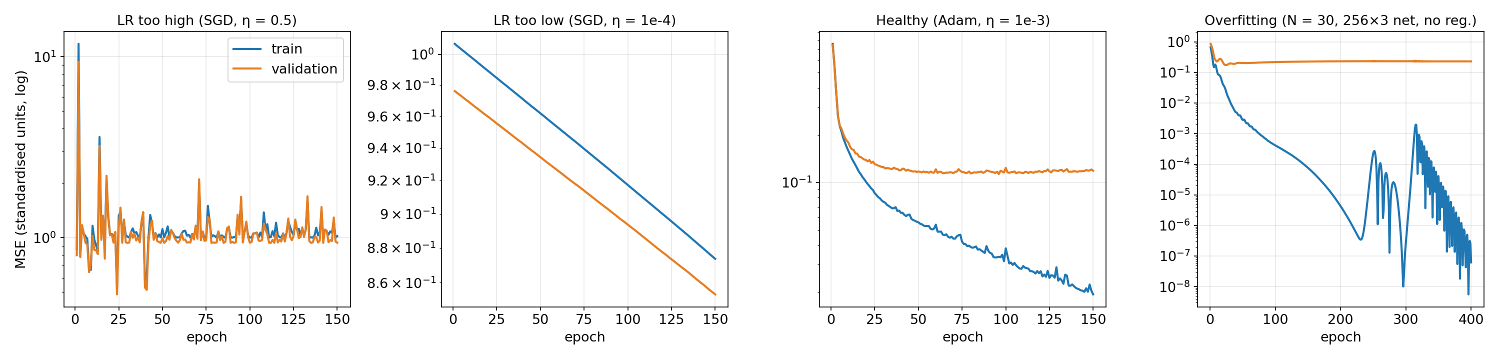
Real training runs of a small MLP on a Hall–Petch-type dataset (train = blue, validation = orange; always plot both, log scale). LR too high: noisy, no progress. LR too low: smooth but painfully slow. Healthy: fast drop, validation plateaus close to train. Overfitting: training loss → 0 while validation stalls — a large net on \(N=30\) memorises. Figure: img/make_figures.py.

• Go panel by panel and ask the class for the diagnosis before revealing the caption. This is exam material: “given this curve, what would you change?”
• LR too high → lower η by 3–10×, or add clipping. LR too low → raise η (LR finder next slide). Healthy → early stopping at the validation plateau. Overfitting → more data, regularisation, smaller network — and check the baseline ladder.
• The one point to land: always plot train and validation loss on a log scale, from epoch 0. The training curve alone cannot distinguish “healthy” from “overfitting”.
• Misconception to preempt: “a diverging validation loss means a bug.” Usually it means overfitting. A diverging training loss means an optimisation problem (LR, init, exploding gradients) or a bug.
• EM anchor: with a GroupKFold-by-specimen split (Week 4), a large train/val gap often signals specimen-specific features being memorised — the validation curve is your leakage detector too.
• Transition: “How do we pick a learning rate without guessing?”

Learning-rate range test (“LR finder”)

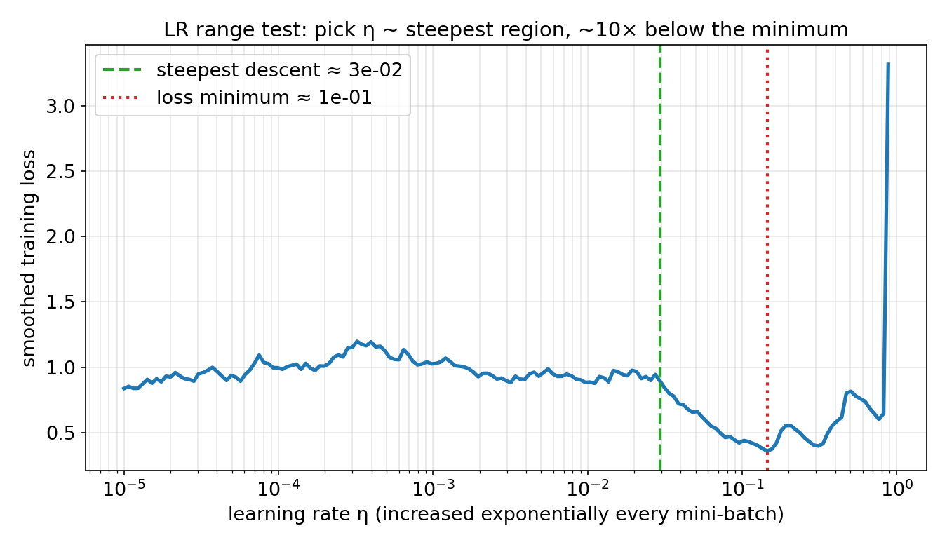
LR range test on a small MLP: η increases exponentially every mini-batch; the loss is flat for tiny η, drops steeply in a useful window, and diverges when η is too large. Figure: img/make_figures.py.

• Multiply η by a constant every mini-batch, record the loss, stop at blow-up Smith, Leslie N., (2017).
• Pick η in the steepest region, 3–10× below the minimum.
• One short pass — far cheaper than a grid search.

• Logic: at each step the model is effectively trained for one mini-batch at learning rate η. Where the loss falls fastest, η is large enough to make progress but small enough to be stable.
• The one point to land: the LR is the single most important hyperparameter. The range test turns a guess into a one-minute measurement. Re-run it when you change architecture, batch size or optimiser.
• Misconception to preempt: “choose the η at the loss minimum.” There the model is already on the edge of instability. Back off by 3–10×.
• Adam’s default η = 1e-3 is usually a reasonable start; the range test tells you whether your problem is unusual.
• Transition: “Before any long run: sanity checks that catch most bugs in minutes.”

Sanity checks before a long run

1. Initial loss: standardised regression MSE ≈ 1; \(K\)-class softmax \(\mathcal{L}_0 \approx \ln K\) (1.39 for 4 phases).
2. Overfit one batch: ~16 samples, no regularisation → training loss must reach ≈ 0. If not, it is a bug, not lack of data.
3. Gradient check custom losses/layers.
4. Per-layer gradient norms: early ≪ late → vanishing; growing → exploding.
5. Look at predictions: parity plots, masks, worst errors.

• These checks save days in the miniproject. Put a checkmark next to each in your notebook.
• The one point to land: overfit-one-batch is the fastest bug detector in deep learning. It separates “my code is broken” (labels shuffled, zero_grad missing, wrong loss, frozen layers) from “my model does not generalise” — two problems with completely different fixes.
• Misconception to preempt: “overfitting one batch is bad.” Here it is the goal — a test that the optimisation machinery works.
• The \(\ln K\) check: with random init the softmax output is roughly uniform, so \(-\ln(1/K) = \ln K\). Binary with sigmoid: \(\ln 2 \approx 0.69\). Far off → wrong loss, wrong labels or bad init.
• EM anchor: a common miniproject bug is shuffling images and masks independently in a custom dataset — overfit-one-batch catches it in two minutes.
• Transition: “With a network that trains, the remaining enemy is overfitting.”

Overfitting: early stopping and dropout

• A 2 × 64 MLP has > 5000 parameters — often more than the EM samples you have.
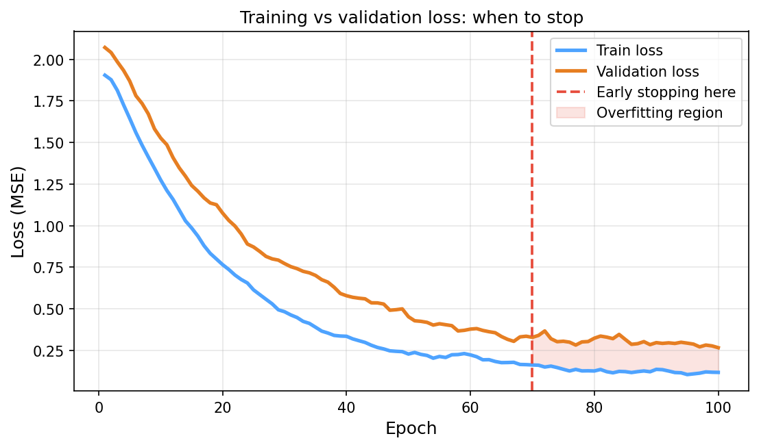
• Cures, in order: more data · early stopping (keep the best-validation epoch) · dropout · smaller network · weight decay.
• Dropout Srivastava, Nitish et al., (2014): zero a fraction \(p \approx 0.2\)–\(0.5\) of hidden units per training pass → no co-adaptation, an implicit ensemble. Off at test time (model.eval()).

• Connect back to Week 4: train/val/test split, GroupKFold, bias–variance trade-off apply unchanged; NNs just have more parameters, so the risk is higher.
• Early stopping: monitor validation loss, save the model at the best epoch — free and the most practical regulariser (the “healthy” panel of the loss-curve slide; an extra early-stopping figure is in the backup).
• Dropout details: PyTorch uses “inverted dropout” — scales by \(1/(1-p)\) during training so nothing changes at test time. Add after hidden layers, not after the output. It is effectively training an ensemble of \(2^N\) thinned networks.
• Misconception to preempt: “dropout always helps.” In small networks or with large \(N\) it only slows convergence. It is a regulariser for high-variance models.
• EM anchor: a deep MLP on 80 HAADF grain-boundary images: training accuracy 100 %, test 55 %. Early stopping at epoch 150 instead of 2000: test 78 %.
• Transition: “Even with perfect regularisation: does the NN actually beat the simpler rungs?”

The baseline ladder: a NN must earn its place

• mean → linear/Ridge → RF/GBM → NN, every rung on the same GroupKFold split with the same preprocessing.
• Tabular descriptors at small/medium \(N\): tree ensembles are very hard to beat Grinsztajn, Léo et al., (2022).
• Raw images/spectra: the NN (with the right inductive bias, Week 7) is the only rung that learns features itself.
• Notebook (Hall–Petch, test \(R^2\)): mean ≈ 0 · Ridge raw 0.80 · MLP 0.65 · RF 0.86 · GBM 0.88 · Ridge on \(1/\sqrt{d}\) 0.91.

• This slide connects today with last week. Draw the Week 5 ladder next to today’s MLP.
• The one point to land: “a neural network” is not a result; “a neural network that beats a tuned RF/GBM on the same GroupKFold split by X” is a result. That is the standard for the miniproject report. Here the NN does not earn its place.
• An MLP is worth it with more data, smooth relationships, or as part of a larger differentiable model.
• Misconception to preempt: “trees are old-fashioned.” On tabular data they remain state of the art — robust to uninformative features and to non-smooth targets, while MLPs are biased towards smooth functions.
• EM anchor: for the Week 5 defect classification on local-environment descriptors a GBM is the expected winner; from raw HAADF patches a CNN (Week 7) is the natural choice.
• Transition: “So when exactly is a deep net the wrong tool?”

When NOT to use a deep net for EM data

• Small tabular data (\(N < 200\) specimens): Ridge or GBM almost always generalises better.
• Known physics (\(H \propto d^{-1/2}\)): embed it rather than learn it.
• Mandatory interpretability: white-box models (Hall–Petch, CALPHAD) when the mechanism is known.
• Images as flat vectors: a dense layer on 1024×1024 pixels needs \(\sim10^9\) weights — wrong architecture → CNN (Week 7).
• Universal approximation says a wide net can represent any continuous function — not that GD finds it, that your data suffice, or that it survives distribution shift.

• Students at MSc level often over-engineer. Spend a moment on each case.
• The one point to land: the right model is the simplest one that explains the data honestly. Complexity is justified by validation, not by trend — and not by the UAT, which is an existence theorem, not a constructive one.
• Misconception to preempt: “a deep net looks more impressive in a report.” The examiner will ask: did you compare to a linear baseline, and did the deep net win on the honest test set?
• Distribution shift: a denoiser trained on Titan data at 300 kV may fail on ARM data at 80 kV because the noise statistics differ — a data problem, not an architecture problem.
• EM anchor: Hall–Petch with 60 samples → analytic \(1/\sqrt{d}\). Steel hardness from 20 compositional features and 5000 samples → MLP can be justified. 4D-STEM with 200 × 200 probe positions of 128 × 128 patterns → CNN (Week 7).
• Transition: “Put it all together into one recipe.”

The complete training recipe

1. Architecture: 2–3 hidden layers, 32–128 units, ReLU.
2. Initialise: He for ReLU (framework default), never zero.
3. Normalise inputs: StandardScaler fit on train only.
4. Sanity checks: initial loss, overfit one batch, LR range test.
5. Train: Adam \(\eta = 10^{-3}\), batch 32–64, early stopping on validation loss.
6. Evaluate honestly: same GroupKFold split, RF/GBM baseline alongside.

• This is the practical recipe students will use in their miniproject. Nothing here is new: every step maps to a concept from Weeks 2–5 or from earlier today.
• Misconception to preempt: “neural networks have their own validation rules.” They do not — GroupKFold, train/val/test split, no leakage apply without exception.
• EM anchor: the Week 6 notebook follows this recipe on the Hall–Petch dataset. A fuller worked scenario (4-feature hardness MLP) is on a backup slide.
• Forward link: Week 7 adds one more step — choosing dense MLP (tabular) vs CNN (images).
• Transition: “Here is the notebook that puts it into practice.”

Self-study notebook: week06_tiny_mlp.ipynb

• Notebook: notebooks/week06_tiny_mlp.ipynb — CPU only, < 1 min.
  • Ridge on \(1/\sqrt{d}\) vs MLP on raw \((d, T)\), plus RF/GBM on the same split.
  • Manual backprop vs autograd vs central differences on the worked example (relative error < \(10^{-8}\)).
  • Exercise: width and activation (ReLU vs tanh).
• — complete before Week 7.

• Point out that the gradient-check part uses exactly the numbers of the worked example: students can compare the printout with their board notes.
• The one point to land: the notebook is the hands-on version of three slides: worked backprop, gradient checking, baseline ladder. The Week 7 CNN notebook assumes you can read a loss curve and trust backward().
• Misconception to preempt: “PyTorch is only for GPUs.” Everything here runs on a laptop CPU in seconds.
• Transition: “Let me summarise.”

Summary: the week in six points

• Neuron \(\sigma(\mathbf{w}^\top\mathbf{x} + b)\); MLP = composed layers; nonlinearity makes depth meaningful. ReLU inside; matched output/loss.
• Backprop = reverse-mode autodiff: store activations, run \(\boldsymbol\delta^{(\ell)} = \sigma'(\mathbf{z}^{(\ell)})\odot\mathbf{W}^{(\ell+1)\top}\boldsymbol\delta^{(\ell+1)}\); weight gradient \(\boldsymbol\delta\,\mathbf{a}^\top\); cost ≈ one forward pass.
• Verify with central finite differences (float64, relative error).
• Trainability: ReLU, He/Xavier init, batch/layer norm keep per-layer factors ≈ 1; clip as a safety net.
• Diagnostics: train + val loss curves, LR range test, initial loss, overfit one batch.
• Honesty: same GroupKFold split, RF/GBM baseline; a NN must earn its place.

• Use this slide as a closing recap and as an orientation for students who fell behind.
• The one point to land: neural networks fit entirely inside the ERM + gradient descent framework from Week 4; backprop makes the gradient cheap; init/normalisation/diagnostics make the optimisation work; the baseline ladder keeps us honest.
• Pacing note: at most 2 minutes; ask for questions before the must-know slide.
• Transition: “The exam-level core, in ten lines.”

Must-know for the exam

1. Dense layer \(\mathbf{a} = \sigma(\mathbf{W}\mathbf{x} + \mathbf{b})\), parameter count \(M(D+1)\); stacked linear layers collapse to one affine map.
2. Output/loss pairs: identity + MSE, sigmoid + BCE, softmax + CE (gradient \(\hat{\mathbf{p}} - \mathbf{y}\)).
3. Hand-compute forward and backward pass of a 2-layer ReLU network (worked example).
4. Delta recursion and \(\nabla_{\mathbf{W}^{(\ell)}} = \boldsymbol\delta^{(\ell)}\mathbf{a}^{(\ell-1)\top}\); backprop costs \(O(W)\), finite differences \(O(W^2)\).
5. Gradient check: central differences, relative error, float64.
6. Vanishing (\(\sigma' \le 0.25\)) / exploding gradients; ReLU, clipping.
7. Zero init fails (symmetry); Xavier \(2/(D_\text{in}+D_\text{out})\), He \(2/D_\text{in}\) — and why.
8. BatchNorm vs LayerNorm: what is averaged, train vs eval, small-batch caveat.
9. Read loss curves; LR range test; initial loss ≈ ln K; overfit-one-batch.
10. Baseline ladder: NN vs RF/GBM on the same GroupKFold split.

• These ten points mirror _shared/mustknow_parts/week06.md. Expect at least one hand-backprop and one “diagnose this loss curve” question.
• Transition: “And next week: what changes when the input is an image?”

Next week (Week 7): CNNs & U-Nets for microscopy

• Problem: a flattened 1024×1024 image into a dense layer needs \(\sim 10^9\) weights — with \(N < 1000\) images the model memorises noise.
• Fix: build in locality and weight sharing → convolution, a sparse, weight-tied matrix multiply.
• Week 7: receptive fields, pooling; VGG → ResNet (skip connections + batch norm — today’s tools); U-Net segmentation with Dice/IoU; saliency and Grad-CAM.
• Inductive-bias arc: MLP (no structure) → CNN (grid, W7) → GNN / transformer (graphs and sets, W10).

• This is the forward-link slide. Its job is to leave students motivated for Week 7 by naming the precise problem that CNNs solve.
• The one point to land: the CNN is not a different paradigm from the MLP — it is an MLP with two structural constraints added. Everything from today (forward pass, activation, backprop, loss minimisation) carries over unchanged.
• Misconception to preempt: “convolution is a completely different operation from matrix multiply.” It is a sparse, weight-shared matrix multiply.
• EM anchor: the FAU group’s phase-retrieval network for 4D-STEM uses a U-Net. The MLP trained today is its conceptual building block.
• Pacing note: 2 minutes. Give them a compelling reason to come back next week and close.
• Transition: “Try the notebook before Week 7. Everything from today — backprop, init, loss curves — will be hands-on.”

Continue

• ← Previous: Unit 05 — From images to features: descriptors & tree ensembles
• → Next: Unit 07 — CNNs & U-Nets for microscopy
• All courses

Backup slides

Material for questions and self-study — not part of the 90-minute lecture path.

The information bottleneck: from micrograph to scalar

• A 1024×1024 BSE micrograph has \(\sim 10^6\) pixels; an ASTM grain-size number discards \(\sim 10^6{:}1\).
• A hand-crafted descriptor answers exactly the question it was designed for, and nothing else Sandfeld, Stefan et al., (2024).
• Learned representations let the network decide which aspects of the field matter for the target — adaptive, not blind compression — given enough data and honest validation.

• JPEG compresses all images the same way; a learned autoencoder compresses depending on the training set. Neither is universally better.
• Irrelevant information (detector noise, beam drift) hurts if included — the question is compression quality, not ratio.
• PCA (Week 3) is already a linear learned representation; autoencoders (Week 9) are the nonlinear, explicit version.

ADALINE and gradient descent on a neuron

• History: MCP neuron (1943, fixed weights) → Perceptron (1957, error-correction rule, hard threshold) → ADALINE (1960): continuous output, MSE, gradient descent: \[\nabla_\mathbf{w}\hat{R} = \frac{2}{N}\mathbf{X}^T(\mathbf{X}\mathbf{w} - \mathbf{y})\]
• This is exactly the Week 4 linear-regression GD update, at the level of a single neuron.

• Gradient-based learning is not new with deep learning — ADALINE = linear regression with a GD optimiser. Fitting an EELS background polynomial by MSE gradient descent is ADALINE applied to spectroscopy.

MLPs learn hierarchical features

• Layer 1: simple combinations of raw features (“large grain AND high temperature”).
• Layer 2: combinations of those (“… AND low Cr fraction”). Output: linear map on the last hidden layer.
• Universal approximation: one wide hidden layer can approximate any continuous function Goodfellow, Ian et al., (2016); in practice depth is more parameter-efficient than width.

• Depth buys representational efficiency: some functions need exponentially fewer neurons in a deep net than in a shallow one.
• EELS example: layer 1 energy-window responses, layer 2 spectral ratios, layer 3 oxidation-state indicators.

Historical activations: step, sigmoid, tanh

• Step \(\mathbb{1}[z \ge 0]\): derivative zero everywhere — no gradient learning (MCP neuron, original perceptron).
• Sigmoid \((1+e^{-z})^{-1}\): \(\sigma' = \sigma(1-\sigma) \le 0.25\), saturates for \(|z|>3\); dominated 1986–2012; today only at binary outputs.
• Tanh: zero-centred, \(\tanh' \le 1\), still saturates. ReLU (AlexNet, 2012): gradient exactly 1 for \(z>0\) — made 10–100-layer networks trainable.

• At \(z = 5\): \(\sigma'(5) \approx 0.007\); over 8 layers \(0.007^8 \approx 6\times10^{-17}\).
• Dying ReLU (units stuck at 0) motivates Leaky ReLU / GELU — fine-tuning concerns, not beginner concerns.

Training loss and early stopping

Training loss (blue) and validation R² (orange) versus epoch. Training loss decreases monotonically; validation R² peaks around epoch 70 and then levels off — the optimal stopping point.

• Monitor validation loss (or R²), not training loss; save the model at the best validation epoch. “Training until convergence” means until validation stops improving.

MLP for materials property prediction: a complete example

• Problem: Vickers hardness from grain size, processing temperature, Cr and Mn fraction.
• Pipeline: StandardScaler (train only) → 4 → 64 → 64 → 1, ReLU, identity output → Adam \(\eta = 10^{-3}\), batch 32, early stopping (n_iter_no_change = 30).
• Baseline: Ridge and RF/GBM on the same features and GroupKFold split; if the MLP does not win, the data are too small or the relation too simple.

• Stainless-steel example: 13 raw features, N = 400, GroupKFold over heats: MLP \(R^2 = 0.82\) vs Ridge 0.76 — a modest but real gain that justifies the complexity.

References

Materials data science, Stefan Sandfeld & others.

Deep learning, Ian Goodfellow, Yoshua Bengio, & Aaron Courville.

Learning representations by back-propagating errors, Nature, David E. Rumelhart, Geoffrey E. Hinton, & Ronald J. Williams.

Automatic differentiation in machine learning: A survey, Journal of Machine Learning Research, Atılım Güneş Baydin, Barak A. Pearlmutter, Alexey Andreyevich Radul, & Jeffrey Mark Siskind.

Pattern recognition and machine learning, Christopher M. Bishop.

Understanding the difficulty of training deep feedforward neural networks, International conference on artificial intelligence and statistics (AISTATS), Xavier Glorot & Yoshua Bengio.

Delving deep into rectifiers: Surpassing human-level performance on ImageNet classification, International conference on computer vision (ICCV), Kaiming He, Xiangyu Zhang, Shaoqing Ren, & Jian Sun.

Batch normalization: Accelerating deep network training by reducing internal covariate shift, International conference on machine learning (ICML), Sergey Ioffe & Christian Szegedy.

Layer normalization, arXiv preprint arXiv:1607.06450, Jimmy Lei Ba, Jamie Ryan Kiros, & Geoffrey E. Hinton.

Group normalization, European conference on computer vision (ECCV), Yuxin Wu & Kaiming He.

Cyclical learning rates for training neural networks, 2017 IEEE winter conference on applications of computer vision (WACV), Leslie N. Smith.

Dropout: A simple way to prevent neural networks from overfitting, Journal of Machine Learning Research, Nitish Srivastava, Geoffrey Hinton, Alex Krizhevsky, Ilya Sutskever, & Ruslan Salakhutdinov.

Why do tree-based models still outperform deep learning on tabular data?, Advances in Neural Information Processing Systems (NeurIPS), Datasets and Benchmarks Track, Léo Grinsztajn, Edouard Oyallon, & Gaël Varoquaux.