ECLIPSE Presentations – Data Science for Electron Microscopy Week 7: CNNs & U-Nets for microscopy

Recap: Week 6 and today’s question

Week 6: neural networks from first principles — perceptron, MLP, activations, softmax/cross-entropy, autograd and backprop, initialisation, batch/layer norm, training diagnostics.
Core insight: a network is empirical-risk minimisation by gradient descent on a composition of learnable maps; backprop gives \(\nabla_\theta \hat{R}\) for free.
Gap: an MLP flattens every image into a vector. A 1024×1024 HAADF image into one dense layer with 1000 neurons already needs one billion weights — and the top-left and bottom-right pixels are unrelated inputs.
Today’s question: how do we build spatial structure into the architecture — locality, “same feature anywhere”, hierarchy — and how do we check what the trained network actually looks at?
Answer: convolutional networks, U-Nets for per-pixel segmentation, and saliency-type explanations.

Road map, learning outcomes and self-study

Road map (≈90 min)

Why MLPs fail on images
Convolution: kernels, stride/padding, channels
Weight sharing, equivariance vs invariance, symmetry
Pooling, receptive field, hierarchy
Architectures: LeNet → AlexNet → VGG → ResNet
U-Net segmentation: IoU/Dice, class imbalance, validation, EM cases
Explainability: saliency, Grad-CAM, occlusion, shortcuts
Failure modes, checklist, notebook, Week 8 preview

After today you can …

compute output shapes, parameter counts and receptive fields of a CNN;
distinguish translation equivariance from invariance and say which a task needs;
explain why skip connections make deep nets (ResNet) and sharp masks (U-Net) possible;
evaluate a segmentation with IoU/Dice and handle class imbalance;
produce and critically read saliency, Grad-CAM and occlusion maps.

Orientation only — 1–2 minutes. Point out the two anchors: the U-Net section (the workhorse for EM segmentation) and the shortcut-learning demo (the trust lesson).
Self-study: notebooks/week07_cnn_segmentation.ipynb — kernels, an equivariance check, a tiny U-Net trained on synthetic particle images on CPU, saliency on a failure case, and the shortcut demo. Pointer slide near the end.
Timing plan (90 min):
- 0–4 min: recap + road map (2 slides)
- 4–7 min: §1 why MLPs fail (2 slides)
- 7–17 min: §2 convolution, grain example, formula, kernels, stride/padding/channels (5 slides)
- 17–26 min: §3 weight sharing, equivariance, rotations, three routes to symmetry, inductive bias (5 slides)
- 26–34 min: §4 pooling, max-pool example, receptive field, feature hierarchy (4 slides)
- 34–42 min: §5 timeline, LeNet/AlexNet, VGG, ResNet (4 slides)
- 42–58 min: §6 U-Net (2), metrics, class imbalance, tiny U-Net, validation, two EM case studies (8 slides)
- 58–70 min: §7 explainability — why, three methods, shortcut demo, segmentation failure, sanity checks (5 slides)
- 70–75 min: §8 failure modes + checklist, notebook pointer (2 slides)
- 75–81 min: summary, must-know, Week 8 teaser (3 slides)
- 81–90 min: questions / slack (≈5 min) + buffer for discussion of the shortcut demo
Backup slides after the “Continue” slide (residual-block details, Au nanoparticle case study) — use on request.
Transition: “Start with the concrete problem — why does a plain MLP fail on microscopy images?”

The parameter explosion: a concrete count

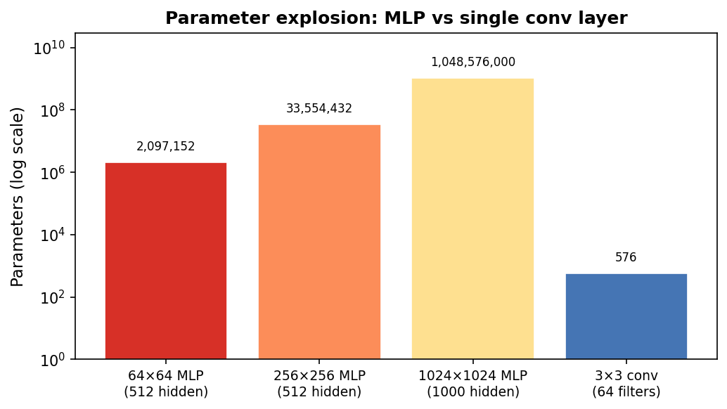
MLP parameter count vs a single convolutional layer for images of increasing size. Note the log scale. A 1024×1024 image with 1000 hidden neurons requires ~10⁹ weights; 64 conv filters of size 3×3 require only 576.

Walk through the four bars explicitly. Left three: MLP on a 64×64, 256×256, and 1024×1024 image. Right: a single convolutional layer with 64 filters of size 3×3.
The one point to land: the CNN bar is not visible at this scale — it is down at 576 parameters while the MLP is at 10⁹.
Misconception to preempt: “more parameters = better.” With small EM datasets (50–500 images), 10⁹ parameters means perfect memorisation of the training set and zero generalisation.
EM anchor: a real 4D-STEM scan is 512×512 real-space × 128×128 momentum-space. Even the spatial slice is 262,144 pixels. No sane practitioner runs a dense MLP on that.
Forward link: weight sharing is the mechanism that collapses 10⁹ to 576 — that is the next conceptual pivot.
Transition: “The parameter count is one problem. The second problem is spatial blindness.”

Three failures of MLPs on images

Problem	MLP behaviour	CNN fix
Parameter explosion	\(D \times M\) weights per layer	\(C_{out}(C_{in}k^2+1)\) kernel weights
No spatial structure	flattened: neighbours become unrelated inputs	local receptive field: a \(k \times k\) patch
No translation awareness	a shifted precipitate is a new input vector	weight sharing: one kernel applied everywhere

CNNs are MLPs with locality and weight sharing built in as hard constraints.

Spatial structure: draw a 4×4 image flattened to a vector of 16 numbers. Ask: “Which two numbers were neighbours in the image?” You cannot tell from the vector. After flattening, pixel (100,100) and (200,200) are unrelated input coordinates — yet a grain boundary or an atomic column is defined by its immediate neighbourhood (a 1–3 nm boundary strip is decided by the 10–20 pixels around it).
Translation: if a precipitate moves 5 pixels, the MLP sees a completely different input vector and must have learned the same pattern at every position. “Where’s Waldo”: you scan with a template, you do not memorise where Waldo was last week. The property we want is translation equivariance: shift the input → the feature response shifts by the same amount.
Misconception to preempt: “convolution gives translation invariance.” Conv layers give equivariance; invariance comes from pooling / global average pooling (later today).
Misconception to preempt: “CNNs are always better than MLPs.” For tabular, non-spatial data (composition, temperature) MLPs or linear models are often preferable.
The one point to land: locality + weight sharing = convolution. Everything else (padding, stride, pooling, channels) is implementation detail.
EM anchor: the spatial correlation CNNs exploit is the physics-driven correlation from Week 2 (sampling, Nyquist): nearby pixels sample the same continuous field.
Transition: “Let us now look at the core operation — convolution.”

Convolution: a sliding feature detector

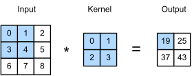
Two-dimensional cross-correlation (the operation CNNs actually use): the 3×3 kernel slides over the input; at each position nine products are summed into one output value.

Slide a small kernel (e.g. 3×3 weights) across the image.
At each position: multiply with the patch, sum → one output value.
Output = feature map: how strongly the kernel’s pattern appears at each location.
\(C_{out}\) kernels in parallel → \(C_{out}\) feature maps.

Narrate one output value explicitly: “align the 3×3 kernel at position (i,j), multiply the 9 overlapping pixels by the 9 kernel weights, sum the 9 products → one number. Slide one pixel to the right; repeat.”
The one point to land: the sliding gives locality (only a local patch is used) AND translation equivariance (the same kernel visits every location).
Misconception to preempt: “convolution flips the kernel.” That is strict mathematical convolution. CNN libraries implement cross-correlation (no flip). Since kernels are learned, the distinction does not matter.
Misconception to preempt: “this is slow.” GPUs evaluate all output positions in parallel with BLAS-level matrix operations.
EM anchor: a 3×3 “bright centre, dark surround” kernel on a HAADF image responds wherever an atomic column is — a column feature map.
Transition: “Let me show this on a synthetic grain image.”

Convolution on a synthetic grain image

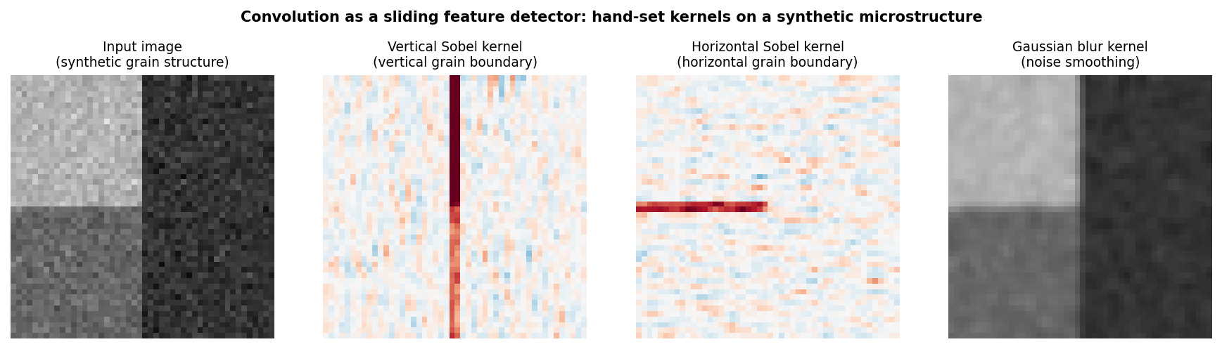
Convolution applied to a synthetic two-grain microstructure. Left: input image (two grains with different intensities, separated by vertical and horizontal boundaries). Centre-left: vertical Sobel kernel responds strongly at the vertical grain boundary. Centre-right: horizontal Sobel responds at the horizontal boundary. Right: Gaussian blur smooths noise. All kernels are 3×3; weights are hand-set, not trained.

Point out explicitly: the two feature maps highlight different boundaries — vertical Sobel fires at the vertical boundary, horizontal Sobel fires at the horizontal boundary. Neither is a correct “grain boundary detector” by itself; you need both in combination.
The one point to land: one 3×3 kernel produces one feature map. A CNN uses many kernels simultaneously, building a richer description.
Misconception to preempt: “CNNs apply edge detectors.” At the first layer, some learned kernels do resemble Sobel. But deeper layers learn highly abstract detectors that do not resemble any named filter.
EM anchor: in a STEM experiment, you might want one feature map for atomic-column positions, one for the background, one for defect signatures. A single convolutional layer can extract all three simultaneously.
Transition: “Let us look at specific hand-set kernels to build intuition before we let the network learn them.”

The discrete convolution formula

For input image \(I\) and kernel \(K\):

\[ (I \star K)_{m,n} = \sum_{a=-\Delta}^{\Delta}\sum_{b=-\Delta}^{\Delta} K_{a,b}\,I_{m+a,\, n+b}, \qquad \Delta = (k-1)/2 \]

Only pixels within \(\pm\Delta\) of \((m,n)\) contribute → local.
\(k^2\) weights, independent of image size \(H \times W\), reused at every \((m,n)\) → weight sharing.

Kernels as feature detectors

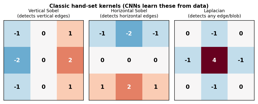
Three classic 3×3 kernels. Left: vertical Sobel — responds to left–right intensity changes. Center: horizontal Sobel — responds to top–bottom changes. Right: Laplacian — responds to any local intensity peak or boundary. Numbers are the kernel weights.

In a trained CNN, the network discovers these (and more complex) filters automatically from labelled examples — no manual kernel design needed.

Name the sign pattern in each kernel. Vertical Sobel: positive on one column, negative on the other → fires at a sign change from left to right. Ask students: “what happens if you flip the sign pattern?” Answer: detects the opposite edge polarity.
The one point to land: these hand-set kernels show what convolution can detect. The power of CNNs is that they learn kernels adapted to the specific task — grain boundary detection, atomic column location, pore segmentation.
Misconception to preempt: “deep CNNs look like Sobel at every layer.” Only the first layer occasionally learns Sobel-like patterns. Deeper layers learn combinations of earlier features that cannot be visualised as simple kernels.
EM anchor: the Laplacian kernel fires at atomic columns (bright spots surrounded by dark background) and at defects — naturally suited to HAADF atomic-resolution images.
Forward link: the notebook lets students hand-set kernels to detect a chosen grain-boundary type — connect this to the Sobel/Laplacian discussion here.
Transition: “Three details control how a convolution layer changes image size: stride, padding, and multiple channels.”

Stride, padding, channels: output size and parameter count

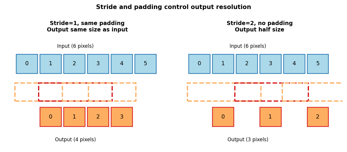
Stride 1 with same-padding (left): output has the input size. Stride 2 (right): the kernel skips every other position, halving spatial resolution.

\(H_{out} = \left\lfloor\frac{H + 2p - k}{s}\right\rfloor + 1\): \(k=3, p=1, s=1\) keeps \(H\) (“same” padding); \(s=2\) halves it.
Kernel tensor \(C_{out}\times C_{in}\times k\times k\) → \(C_{out}(C_{in}k^2+1)\) parameters — independent of \(H, W\): the same network runs on 256² and 4096² images.
EM multichannel inputs: EELS/EDS spectrum images, multi-segment detector stacks.

Concrete numbers: “64×64 image, k=3, p=1, s=1 — H_out?” (64.) “k=3, p=0, s=2?” (31.)
Parameter example: 64 input channels, 128 output channels, 3×3 kernel → 128×(64×9+1) = 73,856 parameters. A dense layer on a 256² image with 128 outputs has 8.4 M — 114× more.
After a layer with \(C_{out}\) kernels the tensor is \(H_{out}\times W_{out}\times C_{out}\) — one feature map per kernel. Beyond layer 1, channels are abstract learned features, not colours.
Stride is the main downsampling tool in modern CNNs (ResNet uses stride-2 convolutions at stage transitions).
Padding options: zero, reflect (natural for real-space HAADF), circular (periodic signals such as diffraction patterns), replicate.
EM anchor: an EELS spectrum image with 1024 energy channels is a 1024-channel input; a conv layer learns spatially localised spectral signatures.
Transition: “Now let us make precise why weight sharing is such a powerful inductive bias.”

Weight sharing: the key efficiency principle

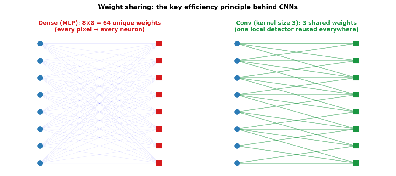
Dense layer (left): every input node connects to every output node — \(n_{in} \times n_{out}\) unique weights. Conv layer (right): the same 3-weight kernel connects each output node to only a local neighborhood of inputs — 3 shared weights total (for the 1-D case shown).

Name the numbers. For the 1-D example shown: 8 inputs × 8 outputs = 64 weights in the dense case. 3-weight conv kernel shared across 8 positions = 3 weights. Factor of 21.
The one point to land: weight sharing is not just an efficiency trick — it encodes a physical assumption. A grain boundary looks the same in the top-left corner and the bottom-right corner of the field of view. The same kernel should detect it in both places.
Misconception to preempt: “fewer parameters = weaker model.” CNNs are empirically more expressive than dense MLPs at the same parameter count on spatial data, because the inductive bias is well-matched to the signal structure.
EM anchor: in HAADF imaging, atomic columns form a repeating pattern across the entire field of view. Learning one column-detector kernel and reusing it everywhere is physically optimal — and exactly what the network does.
Transition: “Weight sharing gives us equivariance — let us be precise about what that means.”

Translation equivariance as an inductive bias

Translation equivariance: if the input shifts by \(\delta\) pixels, the feature map shifts by \(\delta\) pixels — the detector response follows the feature.
Formally: \(f(T_\delta X) = T_\delta f(X)\) for a spatial shift \(T_\delta\).
Translation invariance (different!): \(f(T_\delta X) = f(X)\) — the prediction ignores the shift. Built by pooling, striding, global average pooling.

Equivariance preserves “where.” Invariance discards “where” and keeps only “what.”

Clarify the equivariance vs invariance distinction explicitly. Equivariance is what conv layers give you. Invariance is what you want for image-level classification (does this image contain a precipitate, yes/no). Segmentation tasks need equivariance, not invariance — the output mask must track the position.
The one point to land: architecture choice (conv vs pooling) determines whether you preserve or discard positional information. This is a design choice aligned with the task.
Misconception to preempt: “data augmentation (random crops, flips) trains invariance.” Augmentation helps, but the architectural bias from pooling/striding is what gives the fundamental invariance property.
EM anchor: grain boundary segmentation (U-Net, coming soon) needs equivariance. Defect present/absent classification can discard position. Architecture choice should match the task.
Transition: “Translations are only one symmetry. What about rotations and mirrors?”

Beyond translation: rotations and mirrors in EM

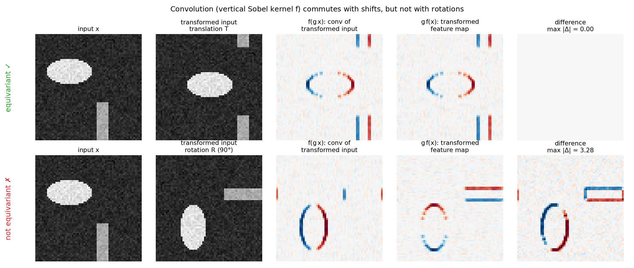
Numerical check with a vertical Sobel kernel \(f\). Top: shifting the input and then convolving equals convolving and then shifting (difference exactly zero). Bottom: for a 90° rotation the two orders differ — the kernel only “knows” vertical edges. Generated by img/make_figures.py.

Walk the two rows. Row 1: \(f(Tx) = Tf(x)\) exactly (circular padding) — this is the equivariance that weight sharing buys. Row 2: \(f(Rx) \ne Rf(x)\); the rod that was vertical is now horizontal and the vertical-edge detector is blind to it.
The one point to land: a plain CNN is equivariant to translations only. It is neither rotation- nor mirror-equivariant, and it is not scale-equivariant either (the scale-sensitivity failure mode later today).
EM anchor: crystal grains appear at arbitrary in-plane orientations; a specimen can be loaded rotated; diffraction patterns have point-group symmetry. For all of these the physics says “the answer should rotate with the input” — the architecture does not know that.
The notebook reproduces this check in PyTorch (Part 4) and asks whether the isotropic Laplacian kernel is 90°-rotation-equivariant (it is — because the kernel itself is symmetric).
Transition: “So how do we get rotation robustness?”

Getting symmetry: three routes

For a group \(G\) of transforms: equivariant \(f(g\cdot x) = g\cdot f(x)\) (masks, denoised images); invariant \(f(g\cdot x) = f(x)\) (phase label).
Route 1 — augmentation: train on rotated/flipped copies; approximate symmetry is learned (Week 8).
Route 2 — test-time augmentation: average predictions over the 8 rotations/flips of \(D_4\) (un-rotate masks first).
Route 3 — build it in: group-equivariant CNNs share weights across rotations too Cohen, Taco et al., (2016).
Rule: know the symmetry of your task first — then learn it, average over it, or hard-wire it.

Brief version of the MFML symmetry discussion. Keep the group language light — “a set of transforms you can compose and undo”.
Trade-offs: augmentation is cheap and universal but costs data and capacity; TTA is free at training time but 8× cost at inference; group-equivariant layers give exact symmetry with fewer parameters but more engineering.
The one point to land: equivariance is what you want in the layers; invariance (if needed at all) is created at the very end, e.g. by global average pooling. Segmentation needs equivariance throughout.
Misconception to preempt: “augmentation makes the network invariant.” It makes it approximately equivariant/invariant on the training distribution — no guarantee on new data.
EM anchor: for atomic-resolution images with a 4-fold or 6-fold zone axis, D4/D6 test-time augmentation is a two-line trick that typically cleans up segmentation noise.
Forward link: the same symmetry question returns for graphs (permutation invariance) in Week 10 and for atomic environments (rotation-invariant descriptors) from Week 5.
Transition: “Choosing an architecture is choosing which symmetries and assumptions to bake in — that is the inductive bias.”

Inductive bias: encoding what you know

An inductive bias is an assumption baked into the architecture that makes certain functions easy to learn.
MLP (Week 6): no structure — every function of all inputs equally easy; needs the most data.
CNN (today): grid + locality + translation weight sharing.
GNN / transformer (Week 10): graph + permutation symmetry; a transformer is a fully connected graph with learned (attention) edges.
Strong, correct bias helps with small datasets by ruling out physically unreasonable solutions; a wrong bias caps performance.

Pooling and the Conv–Pool block

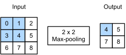
2×2 max-pooling: keep the maximum of each non-overlapping 2×2 region; resolution halves, channel count unchanged.

Max pool: “did the feature appear here?” Average pool: “how strongly on average?” No learned parameters.
2×2 pool halves \(H\) and \(W\) → approximate invariance to small shifts, faster receptive-field growth.
Standard block: Conv → ReLU → MaxPool, channels doubling per stage: 256² input → 16² × 512 after 4 blocks.
Global average pooling at the end → translation-invariant image-level prediction.

Narrate the 2×2 max-pool: take the top-left 2×2 block, keep the largest value, put it at (0,0) of the output; repeat.
The one point to land: pooling gives approximate translation invariance within a window — a precipitate shifted 1 pixel stays in the same window and gives the same pooled output.
Spatial–channel trade-off: 128² × 64 → 64² × 128 → 32² × 256 → 16² × 512. Fine for classification; for segmentation the U-Net decoder must restore the discarded detail — that is what skip connections do.
Misconception to preempt: “average pooling is always worse.” It is better when you care about the average level (how much of this phase is here), not just presence.
EM anchor: max-pool makes an atomic-column detector robust to 1-pixel drift between scans.
Transition: “A worked example.”

Max pooling: a worked example

Input feature map (4×4):

\[ \begin{pmatrix} 1 & 3 & 2 & 4 \\ 5 & 6 & 7 & 8 \\ 3 & 2 & 1 & 0 \\ 1 & 2 & 3 & 4 \end{pmatrix} \]

After 2×2 max-pool (stride 2):

\[ \begin{pmatrix} 6 & 8 \\ 3 & 4 \end{pmatrix} \]

Top-left 2×2 block: \(\max(1,3,5,6)=6\). Top-right: \(\max(2,4,7,8)=8\).

Output size: \(2\times2\) from \(4\times4\) — spatial dimensions halved.
No learned parameters — purely a max operation.
Approximate invariance: if the 6 moved to the adjacent cell (still in the same 2×2 window), the output is unchanged.

Walk through the four quadrants. Top-left: max(1,3,5,6)=6. Top-right: max(2,4,7,8)=8. Bottom-left: max(3,2,1,2)=3. Bottom-right: max(1,0,3,4)=4.
The one point to land: the maximum preserves “was this feature strongly present anywhere in this window?” — appropriate for feature detection where exact position within the 2×2 window does not matter.
Misconception to preempt: “average pooling is always worse.” Average pooling is better when you care about the average activation level (e.g. how much of this phase is in this region), not just whether the feature appeared.
EM anchor: in an atomic-column detector, you want max-pool to be robust to 1-pixel drift of the column within the window. Average-pool would dilute a single bright-column response with its dark background neighbours.
Transition: “Pooling and strided convolutions make the receptive field grow quickly with depth.”

Receptive fields: how much context does one neuron see?

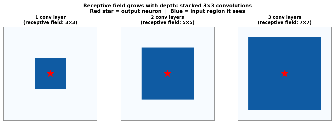
Receptive field of a single output neuron grows with depth. One 3×3 conv layer: 3×3 input region. Two stacked layers: 5×5 region. Three layers: 7×7 region. Red star marks the output neuron; blue region is its receptive field in the input image.

Walk through the three panels. First panel: the output neuron (red star) is determined by a 3×3 patch. Second panel: each neuron in layer 2 was itself determined by a 3×3 patch of layer 1, which was a 3×3 patch of the input — giving a 5×5 input receptive field. Third: 7×7.
The one point to land: depth is how CNNs grow context without expensive large kernels. Three stacked 3×3 layers (3×9=27 params/channel) beat one 7×7 layer (49 params/channel) because there are two extra nonlinearities between them.
Misconception to preempt: “larger kernels always see more.” Two stacked 3×3 layers give the same 5×5 theoretical receptive field as one 5×5 layer — but with fewer parameters and an extra nonlinearity between them, making the representation strictly more expressive. The benefit is not a larger RF; it is parameter efficiency plus added depth.
EM anchor: detecting a dislocation requires seeing context beyond one pixel. A grain triple junction requires seeing ~10–20 nm of context. Pooling rapidly grows the receptive field — by layer 4, one neuron can see a quarter of the image.
Transition: “Growing receptive fields naturally lead to hierarchical features.”

Feature hierarchy: edges → motifs → structures → properties

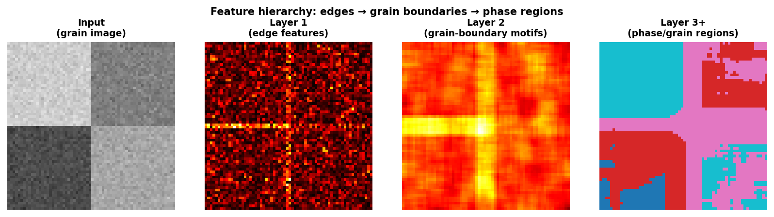
Feature hierarchy on a synthetic grain microstructure. Input (left): two-grain image with boundaries. Layer 1 (centre-left): Laplacian-like edge features highlight all boundaries. Layer 2 (centre-right): neighbourhood-level grain-boundary motifs. Layer 3+ (right): coarse phase/grain-region labels.

Walk through the four panels in order. Point out that each stage is more abstract and coarser in resolution.
The one point to land: this hierarchy is why CNNs are a natural fit for materials images. Microscopy features ARE hierarchical — atoms form columns, columns form grains, grains form microstructures, microstructures encode properties.
Misconception to preempt: “feature maps are always interpretable.” Only Layer 1 features are reliably interpretable as edge/orientation detectors. Deeper features are abstract combinations with no simple physical label.
EM anchor: in HAADF imaging: Layer 1 detects atomic columns. Layer 2 detects local lattice periodicity (grain interior) vs disorder (boundary). Layer 3 detects grain, phase, or defect-cluster regions. Layer 4+ enables phase classification.
Forward link: Grad-CAM (later today) reads out exactly these deep, coarse feature maps to show which region drove a decision.
Mid-lecture checkpoint: “which design choice explains the huge parameter reduction?” (weight sharing) “which explains how a network knows a whole grain is one phase?” (depth + pooling).
Transition: “Let us now look at the major CNN architectures and what each added.”

CNN architectures in one breath: the arc from 1998 to 2015

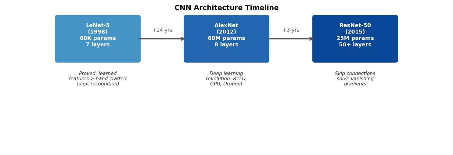
Timeline from LeNet (1998) to AlexNet (2012) to ResNet (2015); VGG (2014) sits between AlexNet and ResNet. Each box states the year, approximate parameter count, depth, and key innovation. Read left to right as increasing depth, scale, and capability.

Read the three boxes together as a story: “LeCun proved learned features beat hand-crafted features for digit recognition. The field then stalled for 14 years while GPUs and datasets grew. AlexNet in 2012 shocked the computer vision community with a 10-percentage-point lead on ImageNet. Then researchers tried to go deeper and hit the vanishing-gradient wall, which ResNet in 2015 solved with skip connections — enabling networks 20× deeper than AlexNet.”
The one point to land: each innovation solved a specific failure mode. LeNet → learning beats hand-craft. AlexNet → scale + ReLU + dropout. ResNet → depth without vanishing gradients.
Misconception to preempt: “you need to know these architectures by name for the exam.” What matters is the progression: what failed, what was added, why. The architecture names are labels for the innovations.
Transition: “LeNet and AlexNet in one slide: the template and the revolution.”

LeNet and AlexNet: the template and the revolution

LeNet-5 LeCun, Yann et al., (1998)

Conv → Act → Pool → Conv → Act → Pool → Flatten → FC → FC → Output
~60,000 parameters; learned features beat hand-crafted ones (SIFT, HOG)
Still the template for small micrograph classifiers

AlexNet Krizhevsky, Alex et al., (2012)

Won ImageNet 2012 by ~10 percentage points
ReLU, dropout, GPU training, ~60 M parameters
Opened the deep-learning era

VGG: deep networks from repeated blocks Simonyan, Karen et al., (2015)

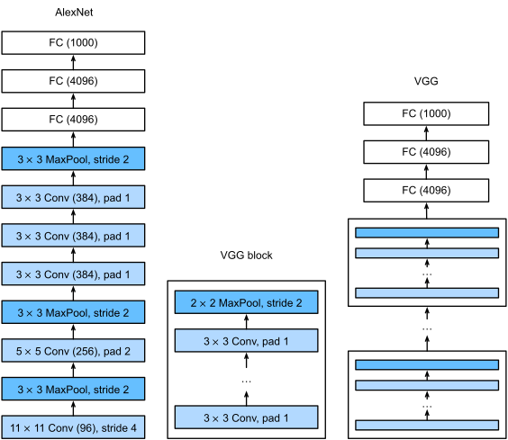
From AlexNet (left) to VGG (right): irregular layers are replaced by repeated blocks of 3×3 convolutions followed by 2×2 max-pooling. Figure: d2l.ai (CC BY-SA 4.0).

VGG block: \(n\times\) (3×3 conv, pad 1, ReLU) → 2×2 max-pool; channels 64 → 128 → 256 → 512.
Why 3×3? Each stacked 3×3 adds 2 pixels of receptive field: three give 7×7 with \(27C^2\) instead of \(49C^2\) weights and two extra non-linearities.
Design lesson: think in blocks, not layers.

ResNet: skip connections make depth trainable He, Kaiming et al., (2016)

ResNet residual block: the main path learns F(x); the skip connection adds x to the output.

Degradation: plain stacks of 20 → 56 layers reach worse training error — not overfitting, an optimisation problem.
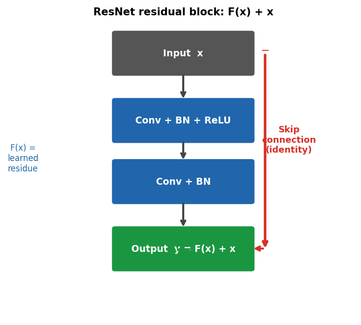
Residual block: \(\mathbf{y} = F(\mathbf{x}) + \mathbf{x}\) — learn only a correction to the identity.
Gradient \(\partial\mathbf{y}/\partial\mathbf{x} = \mathbf{I} + \partial F/\partial\mathbf{x}\): an unattenuated path through every block.
Block: conv–BN–ReLU–conv–BN, add, ReLU.
Skips today: additive (ResNet: optimisation) vs concatenating (U-Net: localisation).

Degradation: He et al. showed that with BatchNorm the gradients are fine, yet the deeper plain net trains worse. Thought experiment: a deeper net could copy the shallow one and set the extra layers to identity — SGD does not find that. Idea: make identity the default.
Connect to Week 6: through 20 sigmoid layers the gradient shrinks by 0.25^20 ≈ 10^-12. ReLU fixed moderate depth; the skip provides a gradient highway for arbitrary depth.
BatchNorm recap (Week 6) Ioffe, Sergey et al., (2015): in CNNs the statistics are per channel over batch × H × W; running averages at inference — remember model.eval().
If shapes change (stride 2, more channels) the skip uses a 1×1 conv. ResNet-18/34/50 = 4 stages, global average pooling + one linear layer (ResNet-18 ≈ 11 M params vs VGG-16 ≈ 138 M). Backup slide has the details.
Misconception to preempt: “ResNet and U-Net skips are the same thing.” ResNet adds \(x\) to help optimisation; U-Net concatenates encoder features to recover where.
EM anchor: “U-Net with ResNet-34 encoder, ImageNet-pretrained” — students can now parse that sentence (the “pretrained” part is Week 8).
Transition: “Classification networks produce one label per image. For EM segmentation we need one label per pixel — that is U-Net.”

U-Net: encoder–decoder for segmentation Ronneberger, Olaf et al., (2015)

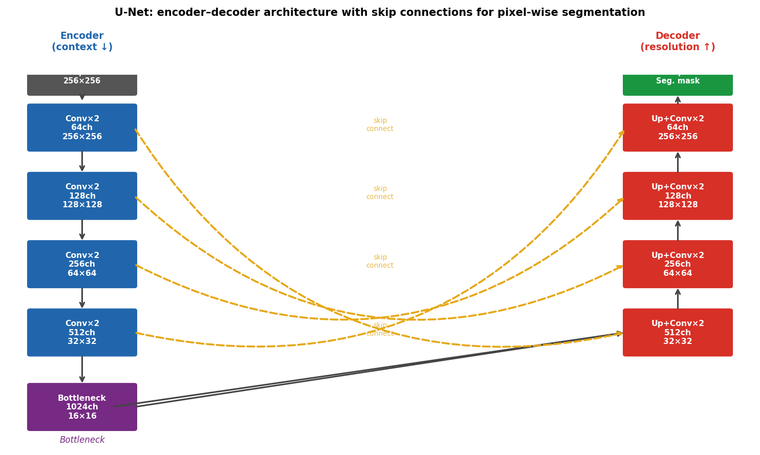
U-Net architecture. Left column (blue): encoder — successive Conv+Pool blocks extract features while halving spatial resolution and doubling channel count. Right column (red): decoder — successive upsample+Conv blocks restore spatial resolution. Yellow dashed arrows: skip connections concatenate encoder features into corresponding decoder levels.

Walk through the architecture from top-left to top-right. “Encoder (blue): each block halves the spatial size and doubles channels — building rich abstract features. Bottleneck (purple): smallest spatial resolution, maximum context. Decoder (red): each block upsamples by 2 and uses a skip connection to bring back fine spatial detail from the corresponding encoder level. Output: same spatial resolution as input, one label per pixel.”
The one point to land: the key innovation is the skip connection that bypasses the bottleneck. Without it, the decoder has to reconstruct fine spatial detail entirely from the compressed bottleneck representation — which is too abstract and loses boundary precision.
Misconception to preempt: “U-Net is only for medical images.” The original paper used biomedical images, but U-Net is now the standard segmentation architecture for any spatially structured prediction — including phase segmentation in TEM and grain tracing in SEM.
EM anchor: the spatial resolution of the output mask (same as input) is critical for measuring grain sizes, locating precipitates, and computing phase fractions. Classification-only CNNs cannot provide this.
Transition: “Let me break down the two paths.”

U-Net: encoder, decoder, per-pixel output

Encoder (context)

(Conv×2 → ReLU → MaxPool) × 4
spatial halves, channels double

Decoder (resolution)

(Upsample → concatenate skip → Conv×2) × 4
final 1×1 conv → \(K\times H\times W\) class scores

Mask = \(\arg\max\) over \(K\) channels; loss = per-pixel cross-entropy (often + Dice), same backprop + Adam.
Without skips, boundary positions are lost in the bottleneck → blurry masks.

Upsampling: bilinear or transposed convolution. Why concatenation, not addition: keep both the fine-detail encoder information (position, texture) and the semantic decoder information.
Loss written out: for binary segmentation, BCE between predicted probability and label at each pixel (m,n), averaged over all pixels in the minibatch. U-Net uses exactly the training machinery from Week 6; only the output head and the loss change.
The one point to land: in segmentation “where?” matters as much as “what?” — skip connections preserve “where.”
Misconception to preempt: “U-Net needs huge training sets.” Ronneberger et al. designed it for ~30 labelled images — ideal for EM.
EM anchor: 4D-STEM phase mapping — input a virtual bright-field image, output phase A / phase B / boundary per pixel.
Transition: “How do we measure whether a mask is good?”

Segmentation metrics: IoU and Dice, not accuracy

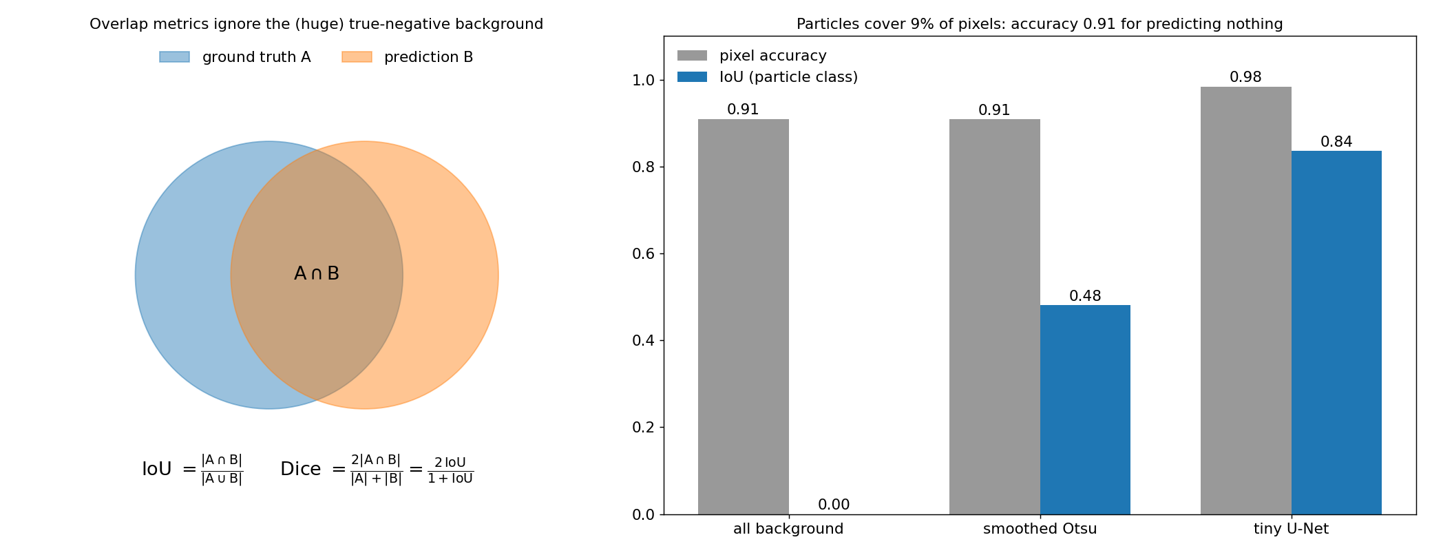
Left: IoU and Dice compare predicted and true foreground sets and ignore true-negative background. Right: on our synthetic particle images (9% foreground) predicting nothing already scores 0.91 pixel accuracy; a smoothed Otsu threshold also scores 0.91 but IoU 0.48; the tiny U-Net from the notebook reaches IoU 0.84. Generated by img/make_figures.py.

Formulas: IoU (Jaccard) \(= |A\cap B|/|A\cup B|\), Dice (F1) \(= 2|A\cap B|/(|A|+|B|) = 2\,\mathrm{IoU}/(1+\mathrm{IoU})\). Dice is always ≥ IoU; they rank models identically on a single image but not always on averages.
The one point to land: pixel accuracy counts the huge, easy background. The all-background “model” and Otsu have the same accuracy (0.91) but completely different usefulness.
Reporting rules: per-class IoU (mean IoU over classes for multi-phase maps); say whether you average per image or pool all pixels; for thin structures (boundaries, cracks) consider a boundary-tolerant metric.
Connect to Week 4 metrics and ML-PC unit 3: same idea as precision/recall under imbalance. Dice is the F1 score on pixels.
Transition: “If the metric must ignore the background, the loss should too.”

Class imbalance: losses that keep the minority visible

Pixel-wise BCE is an average over pixels: with 9% particles, the minority class carries 9% of the loss weight.
Weighted BCE (pos_weight \(=(1-f)/f\)); focal loss Lin, Tsung-Yi et al., (2017) down-weights easy pixels.
Soft Dice loss Milletari, Fausto et al., (2016), with \(p_i=\sigma(z_i)\): \[\mathcal{L}_\text{Dice} = 1-\frac{2\sum_i p_i y_i+\epsilon}{\sum_i p_i+\sum_i y_i+\epsilon}\] normalised by the foreground size → “predict nothing” costs ≈ 1.
BCE + Dice is the default. Notebook: BCE alone collapsed to “all background” (IoU 0.00); BCE + Dice reached IoU 0.84.

Walk the Dice formula: numerator = soft overlap, denominator = soft sizes. It is a ratio, so it cannot be dominated by the background.
The one point to land: the loss encodes what you care about. If you care about the rare class, the loss must say so — metric and loss should be aligned.
The notebook numbers are real (SEED=7, tiny U-Net, CPU): with plain BCE the network found the trivial minimum first; with BCE + Dice the same network, data and optimiser gave IoU 0.84. With longer training BCE would eventually catch up — but the trap is real on budget.
Also sample-level imbalance: crop training tiles around rare objects (oversampling) — but only within the training split.
Misconception to preempt: “Dice alone is best.” Pure Dice has noisy gradients for images with little or no foreground; BCE + Dice is the robust default.
Transition: “What does that tiny U-Net actually produce?”

A tiny U-Net on synthetic particles (the notebook)

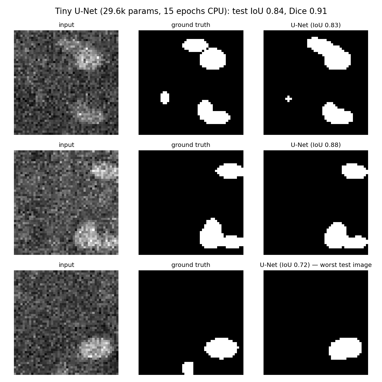
Tiny U-Net (2 levels, 8–16–32 channels, BatchNorm, 29.6 k parameters) trained for 15 epochs on 256 synthetic 48×48 images of bright particles on a textured, unevenly lit support with shot noise. Rows: median, good, and worst test image. The worst case misses a low-contrast particle entirely. Generated by img/make_figures.py (same code and seeds as the notebook).

Numbers (test set from a different generator seed = different “session”): IoU 0.84, Dice 0.91, pixel accuracy 0.98; smoothed Otsu IoU 0.48. Trains in well under a minute on one CPU thread.
The one point to land: even a 30 k-parameter U-Net beats the classical threshold by a wide margin, because it learns to ignore the illumination gradient and the support texture.
Look at the worst image (bottom row): the faint particle is invisible to the model. Always inspect the tail of the per-image IoU distribution, not only the mean.
Ablation in the notebook: removing the skip connections did not hurt here (IoU ≈ 0.84 either way) — the particles are compact blobs and the bottleneck is still 12×12. Skips pay off for thin boundaries and deep U-Nets. Ablations are task-dependent.
Transition: “Before the literature case studies — how do you validate a segmenter honestly?”

Honest validation for segmentation

Tile leakage: cutting one large micrograph into overlapping 256² tiles and splitting the tiles randomly puts neighbouring pixels in train and test → inflated IoU. Split by micrograph, specimen or session (GroupKFold, Week 4).
Label ceiling: measure IoU between two annotators on a subset; a model cannot meaningfully beat that ceiling.
Report per class and per image: mean IoU hides that one rare phase (or the faint particles) is never found.
Downstream quantity: check the number you actually need — particle size distribution, phase fraction, grain count — not just IoU.

EM case study: defects in irradiated steel Roberts, Graham et al., (2019), doi:10.1038/s41598-019-49105-0

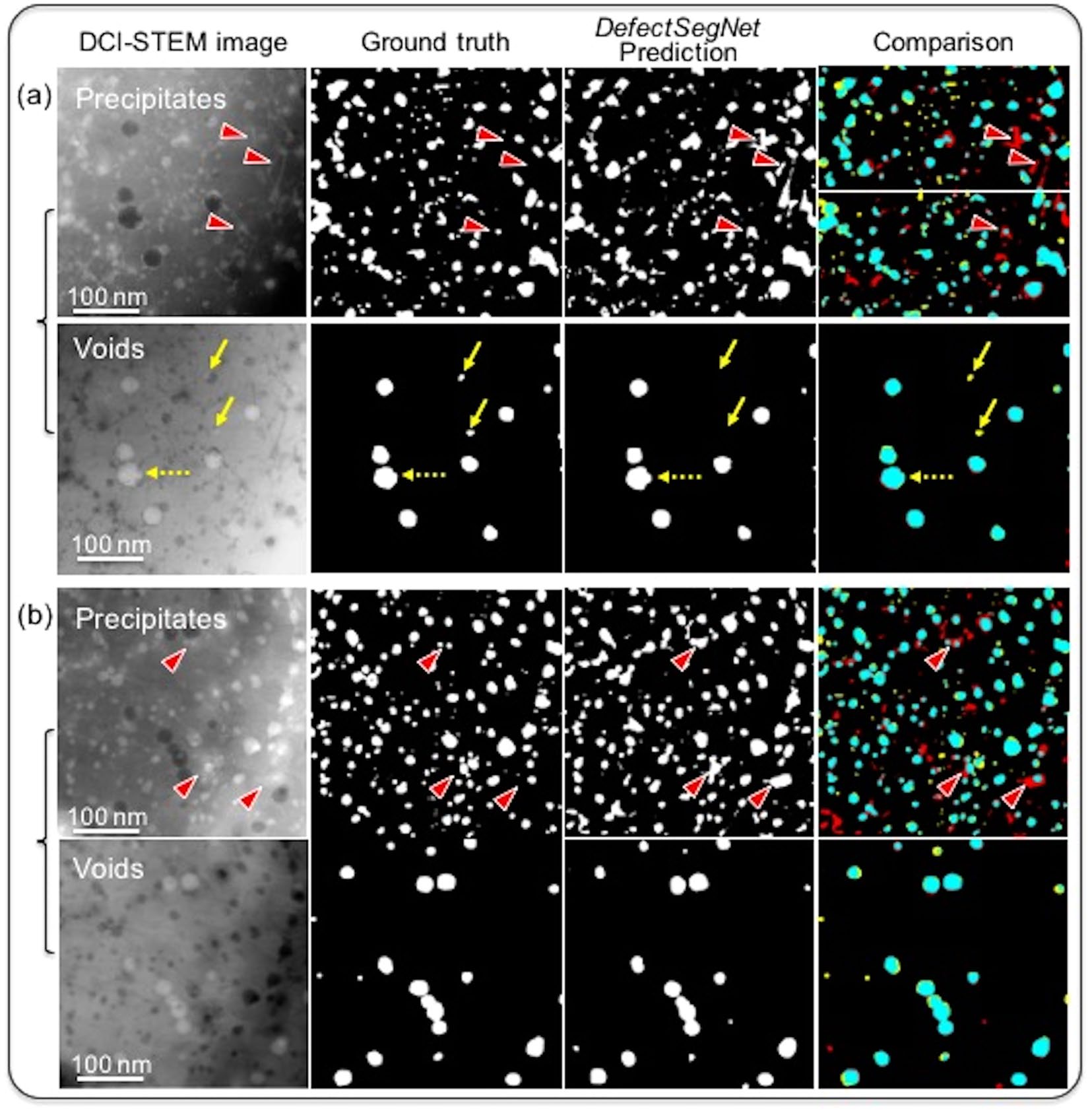
DefectSegNet predictions on STEM (DCI) images of irradiated steel: input, ground truth, prediction and comparison for precipitates and voids. From Roberts, Graham et al. (2019), doi:10.1038/s41598-019-49105-0 (Sci. Rep., CC BY 4.0).

U-Net-type encoder–decoder with dense skip connections; per-pixel labels for dislocation loops, precipitates and voids.
Reaches roughly inter-annotator agreement — beyond that point more model capacity buys nothing; better labels do.

Real-world urgency: post-irradiation reactor steels; very few people can label voids and loops at expert level. The CNN matches them after training on a modest number of labelled images.
Read the figure: four columns = input / human label / CNN / comparison. Most disagreement sits at object boundaries — where humans disagree too.
The one point to land: the annotator floor is the practical ceiling. This connects to the “label ceiling” bullet on the validation slide.
Material from ML-PC unit 4 (case 6).
The Au nanoparticle phase-map case study is on a backup slide.
Labelling cost: a U-Net from scratch on EM data typically needs 50–200 annotated images; transfer/self-supervised pretraining (Week 8) can cut this to 20–50. A compact 4-level U-Net (32→256 channels) has ~7.8 M parameters, the original ~30 M.
Transition: “The second case: no human labels at all.”

EM case study: grain boundaries from synthetic Voronoi labels

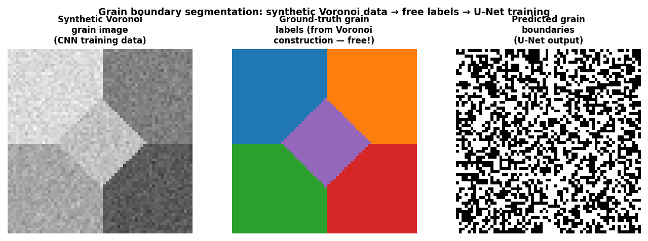
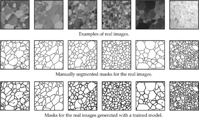
Training: synthetic Voronoi grain image, free ground-truth labels, U-Net predicted boundaries.

Application: the network trained only on synthetic Voronoi images segments grain boundaries in a real SEM polycrystal image.

Voronoi tessellations give perfect labels for free; the boundary topology (“dark strip between two regions”) transfers to real SEM images.

Why explain a CNN in EM?

A segmenter or classifier with 0.99 test accuracy can still be right for the wrong reason — “shortcut learning” Geirhos, Robert et al., (2020).
EM shortcuts: scan-start/detector-edge artefacts, session contrast, scale bars, beam damage tied to one specimen.
Local explanation question: which input pixels drove this particular prediction?
Their job is diagnosis (find shortcuts, understand failures, decide what data to add) — not proof that a model is physically correct.

Three local explanations: saliency, Grad-CAM, occlusion

Gradient saliency Simonyan, Karen et al., (2014): \(S_i = |\partial z_c/\partial x_i|\) — one backward pass w.r.t. the input; pixel-level, noisy; sensitivity, not contribution.
Grad-CAM Selvaraju, Ramprasaath R. et al., (2017): weight the last-conv feature maps by their mean gradient, \(L^c = \mathrm{ReLU}\big(\sum_k \alpha_k^c A^k\big)\), \(\alpha_k^c = \frac{1}{Z}\sum_{i,j}\partial z_c/\partial A^k_{ij}\) — coarse, smooth regions.
Occlusion Zeiler, Matthew D. et al., (2014): slide a grey patch, record the drop \(p_c(\mathbf{x}) - p_c(\mathbf{x}_\text{occ})\) — model-agnostic, forward passes only.
For segmentation: backpropagate from a set of output pixels (e.g. all false positives).

Saliency implementation: x.requires_grad_(True); model(x)[0, c].backward(); S = x.grad.abs() — backprop from Week 6, but w.r.t. the input instead of the weights. No modification of the trained model. Picture: the model is a surface over pixel space; saliency is the local slope. Exam-level: a high value means the prediction is locally sensitive to that pixel — not “this pixel caused the prediction”.
Grad-CAM: the formula is reference, not a derivation to memorise. Resolution = last conv layer (e.g. 8×8, upsampled); class-specific; works for any conv backbone. Connects to the feature-hierarchy slide: the last conv layer holds the most abstract features. Exam question: “how does Grad-CAM differ from input-gradient saliency?” — coarse, smooth, semantically meaningful vs fine and noisy.
Occlusion: measures a global effect (remove a region) instead of a local slope → often crisper. Cost: one forward pass per patch position (notebook: 4×4 patches on 32×32 = 64 passes; a 1024² micrograph with 16² patches = 4096 — use strides and batches). Resolution = patch size. The fill value matters: black in a HAADF image adds a “dark hole”; use the mean or a local blur, and report it.
Transition: “Now put all three to work on the shortcut problem.”

Shortcut learning: same accuracy, different physics

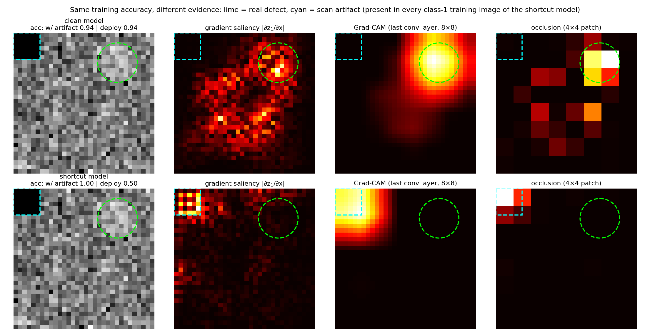
Defect classifiers (class 1 = faint bright disk). The shortcut model was trained on images in which every defect image also had a dark 6×6 corner (a scan-start/detector-shadow artefact); the clean model on the same images without it. Test accuracy with the artefact: 0.94 vs 1.00; deployment accuracy (defects, no artefact): 0.94 vs 0.50. All three methods put the shortcut model’s evidence in the corner. Generated by img/make_figures.py.

Numbers (notebook Part 9, 50 class-1 test images): fraction of attribution mass in the corner (3.5% of the pixels) — clean model 0.00 for all three methods; shortcut model 0.30 (gradient), 0.34 (Grad-CAM), 0.76 (occlusion). Gradient mass on the actual defect: clean 0.19, shortcut 0.03.
The one point to land: on a test set drawn from the same sessions the shortcut model looks better (1.00). Only a shifted test set (0.50 = chance) or an explanation reveals the problem. This is Week 4 leakage in disguise.
The three methods agree on where, differ in sharpness: occlusion is crispest, Grad-CAM smooth and coarse, gradient saliency noisy.
Adapted from the May-2026 explainability week; the artefact is now dark and co-occurs with the real defect, which makes it a genuine spurious correlation.
Remedies: remove/crop the artefact, include artefact images in both classes, randomise acquisition across classes — i.e. fix the data, the explanation only diagnoses.
Transition: “The same idea works for a segmentation network.”

Explaining a segmentation failure

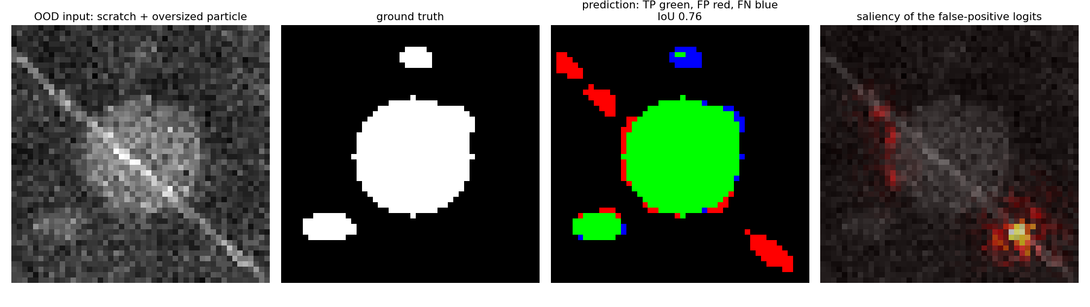
Tiny U-Net applied to an out-of-distribution image with a bright scratch and an oversized particle. Scratch segments become false positives (red); the saliency of the summed false-positive logits sits on the scratch itself. Generated by img/make_figures.py.

Sanity checks and honest limits of saliency

Model-randomisation test Adebayo, Julius et al., (2018): randomise the weights and recompute. If the map barely changes, it shows image structure, not what the model learned (notebook: correlation ≈ 0 — passes).
Fragility Kindermans, Pieter-Jan et al., (2019): simple input transformations (e.g. a constant shift) can change some attribution maps without changing the prediction.
Sensitivity ≠ causation: a coherent map can be coherent about the wrong feature (the corner).
Use them as hypotheses → test them: occlude the suspected region, build a shifted test set, retrain without the cue.

Adebayo et al. showed that several popular methods (e.g. guided backprop) produce almost the same maps for trained and random networks — they are edge detectors. Plain gradient saliency passes the test; the notebook’s Exercise 3 reproduces this (correlation ≈ 0.01, corner mass drops from 0.28 to 0.03).
The EM trap: HAADF images already have strong contrast at atomic columns. A method that just highlights bright pixels will always look plausible on HAADF data. Hence the randomisation check before any explanation goes into a paper or miniproject.
The one point to land: explanations are diagnostic hypotheses. The decisive evidence is an intervention: occlude, shift, retrain.
Forward link: Week 9 (latent-space pitfalls), Week 10 (attention ≠ explanation), Week 11 (uncertainty as a trust gate), Week 13 (the full E1–E6 explainability ladder).
Transition: “Back to practical failure modes of CNNs in EM.”

Failure modes and a practical checklist

Failure modes

Domain shift: other microscope, detector, contrast transfer
Beam-damage artefacts that look like boundaries
Scale: trained at 0.1 nm/px, applied at 0.5 nm/px
Out-of-distribution microstructures

Checklist

Match pixel size between training and inference.
GroupKFold by specimen/session — not random splits.
Look at predicted masks; report per-class IoU/Dice.
Start simple; beat a thresholding baseline first.
Explain before deploying (+ randomisation check).

Failure story: a U-Net for Au nanoparticle segmentation applied to Pt nanoparticles — similar contrast, different lattice spacing — over-segmented the Pt particles into multiple Au-sized objects.
Domain shift fixes: retrain on the target instrument or domain adaptation (Week 8). Beam damage is a uniquely EM failure mode — the CNN cannot distinguish damage from structure unless trained to.
The one point to land: CNNs learn correlations in the training data. Validation on held-out sessions (Week 4) is essential — the shortcut demo is exactly this failure.
“Start simple”: a 4-level U-Net with 32→256 channels often beats a 50-layer ResNet when N < 200 labelled images. A simple, well-validated model the team can debug beats a complex one with marginally better metrics.
Checklist points 2 and 3 echo Week 4 (honest validation) and Week 6 (look at what the model does).
Forward link: augmentation, transfer and self-supervised learning (Week 8) are the main strategies against domain shift and scale variation.
Transition: “Here is this week’s notebook — and where to practise on real data.”

Self-study notebook

notebooks/week07_cnn_segmentation.ipynb

Hand-set kernels (Sobel, Laplacian, Gaussian) as one conv layer
Equivariance check: shift ✓, rotation ✗
Synthetic particle images with free masks, split by “session”
IoU/Dice and the accuracy trap; Otsu baseline (IoU 0.48)
Tiny U-Net, BCE + soft Dice, CPU: IoU 0.84, Dice 0.91
Saliency on an OOD failure (scratch)
Shortcut demo: saliency, Grad-CAM, occlusion; randomisation check

Open in Colab

Runs end-to-end on a CPU in a few minutes.
Exercises: soft-Dice loss, ablations (no skips / no Dice), saliency sanity check.
Real data: MetalDAM (SEM, AM metal, per-pixel labels) via Ai4MatLectures.

MetalDAM (from ai4mat.datasets import ...) is the real-data version of today’s notebook: real class imbalance, label noise and contrast variation. Miniproject-sized exercise: U-Net with 3–4 levels (or ResNet encoder) → per-class IoU with a split by micrograph (split before tiling into 256² crops) → saliency on the worst class → one augmentation that fixes a failure. Needs a GPU (Colab). Ai4Mat also has HRTEM and NEU-DET surface defects for classification with Grad-CAM.
Stress the ablation exercise: plain BCE collapses to “all background” on this imbalanced data — students should see the class-imbalance trap with their own eyes.
The notebook numbers quoted on the slides come from the same code and seeds (img/make_figures.py reproduces the figures).
Transition: “Summary.”

Summary: the week in six points

Convolution = locality + weight sharing: parameters independent of image size, translation-equivariant feature maps.
Equivariance vs invariance: layers are shift-equivariant; invariance comes from pooling/GAP; rotations need augmentation, TTA or group-equivariant layers.
Depth needs design: VGG blocks of 3×3 convs; ResNet identity skips + BN make very deep nets trainable.
U-Net = encoder (context) + decoder (resolution) + concatenating skips (where) → one label per pixel.
Evaluate with IoU/Dice, fight class imbalance in the loss (BCE + Dice, weights), validate by specimen/session.
Explain before trusting: saliency, Grad-CAM, occlusion diagnose shortcuts and failures; sanity-check the explanation itself.

Must-know for the exam

Output size \(\lfloor (H+2p-k)/s\rfloor+1\) and parameter count \(C_{out}(C_{in}k^2+1)\) — independent of \(H,W\).
\(f(T x)=T f(x)\) (equivariance) vs \(f(Tx)=f(x)\) (invariance); CNNs are not rotation-equivariant by default.
Stacked 3×3 convs: receptive field grows by 2 per layer; pooling/stride multiplies the growth.
ResNet: \(\mathbf{y}=F(\mathbf{x})+\mathbf{x}\) eases optimisation; U-Net skips concatenate encoder features to restore localisation.
IoU, Dice (\(=2\mathrm{IoU}/(1+\mathrm{IoU})\)); pixel accuracy is misleading under imbalance; soft Dice / weighted BCE as remedies.
Saliency \(|\partial z_c/\partial \mathbf{x}|\), Grad-CAM (last conv layer), occlusion (model-agnostic); a plausible map can reveal a shortcut, and must pass a randomisation sanity check.

Next week: small data — augmentation, transfer & self-supervision

Next week’s question: you have 30 labelled TEM images. How do you train a reliable CNN?
Physics-respecting augmentation: rotations/flips from the crystal symmetry, Poisson noise at the right dose, drift, scratches — the fix for today’s scratch failure.
Transfer learning: start from a pretrained encoder (e.g. a ResNet) — linear probe vs fine-tune.
Synthetic data & sim-to-real: Voronoi grains, simulated HRTEM — free labels like today’s notebook.
Self-supervised learning & foundation models: SimCLR, masked autoencoders, DINO; SAM / μSAM for microscopy.

Continue

← Previous: Unit 06 — Neural networks & backpropagation
→ Next: Unit 08 — Small data: augmentation, transfer & self-supervision
All courses

Backup slides

Material not covered in the 90-minute lecture path — for questions and self-study.

Residual blocks in practice: BN, stages, and why EM cares

Basic block: conv3×3 → BN → ReLU → conv3×3 → BN, add input, ReLU. If shapes change (stride 2, more channels) the skip uses a 1×1 conv.
Gradient view: \(\frac{\partial \mathbf{y}}{\partial \mathbf{x}} = \mathbf{I} + \frac{\partial F}{\partial \mathbf{x}}\) — the identity term carries the gradient through every block unattenuated.
Stages: ResNet-18/34/50 = 4 stages of residual blocks, stride-2 between stages, global average pooling + one linear layer (no big dense head: ResNet-18 ≈ 11 M params vs VGG-16 ≈ 138 M).
EM use: ResNet backbones are the standard encoder for U-Net-style segmenters and the usual starting point for transfer learning (Week 8).
Skip connections appear twice today: additive (ResNet: ease optimisation) and concatenating (U-Net: restore spatial detail).

Draw the basic block on the board, and the 1×1 projection skip for the stride-2 case.
The one point to land: identity + small correction. Blocks that are not needed can learn \(F\approx 0\) and become near-identity — depth stops hurting.
Misconception to preempt: “ResNet and U-Net skips are the same thing.” Same name, different purpose: ResNet adds \(x\) to help optimisation; U-Net concatenates encoder features to recover where.
EM anchor: literature on nanoparticle/defect segmentation constantly says “U-Net with ResNet-34 encoder, ImageNet-pretrained” — students can now parse every word of that sentence (the “pretrained” part is Week 8).
Transition: “Classification networks produce one label per image. For EM segmentation we need one label per pixel — that is U-Net.”

EM case study: Au nanoparticle phase segmentation

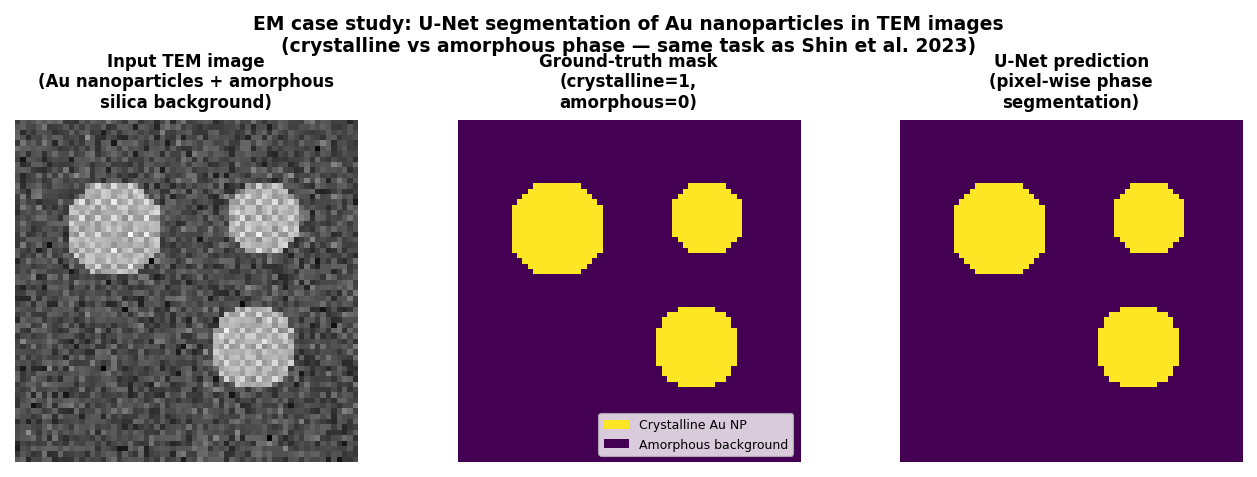
U-Net applied to TEM images of Au nanoparticles on an amorphous support. Left: input TEM image (representative Au-nanoparticle-on-amorphous-support TEM segmentation task). Centre: ground-truth binary mask (crystalline=bright, amorphous=dark). Right: U-Net prediction — pixel-wise classification matching the ground truth closely.

Describe the physical task: “Au nanoparticles are crystalline — they show regular lattice fringes in TEM. The silica matrix is amorphous — shows no periodic structure. The task is to label every pixel as ‘crystalline Au’ or ‘amorphous silica’, producing a quantitative phase map.”
The one point to land: this is exactly the task where U-Net excels — the boundary between phases has a specific local texture signature that the encoder learns, and the exact location of the boundary matters for measuring nanoparticle size distributions.
Misconception to preempt: “we need thousands of labelled TEM frames to train.” In practice, 50–200 carefully labelled frames can train a U-Net for this specific task, especially combined with data augmentation (Week 8).
EM anchor: phase fraction measurement (how much Au vs how much silica?) requires pixel-accurate segmentation — a classification-only CNN cannot provide this.

References

Group equivariant convolutional networks, Proceedings of the 33rd international conference on machine learning (ICML), Taco Cohen & Max Welling.

Gradient-based learning applied to document recognition, Proceedings of the IEEE, Yann LeCun, Leon Bottou, Yoshua Bengio, & Patrick Haffner.

ImageNet classification with deep convolutional neural networks, Advances in neural information processing systems, Alex Krizhevsky, Ilya Sutskever, & Geoffrey E. Hinton.

Very deep convolutional networks for large-scale image recognition, International conference on learning representations (ICLR), Karen Simonyan & Andrew Zisserman.

Deep residual learning for image recognition, Proceedings of the IEEE conference on computer vision and pattern recognition, Kaiming He, Xiangyu Zhang, Shaoqing Ren, & Jian Sun.

Batch normalization: Accelerating deep network training by reducing internal covariate shift, Proceedings of the 32nd international conference on machine learning (ICML), Sergey Ioffe & Christian Szegedy.

U-net: Convolutional networks for biomedical image segmentation, Medical image computing and computer-assisted intervention (MICCAI), Olaf Ronneberger, Philipp Fischer, & Thomas Brox.

Focal loss for dense object detection, Proceedings of the IEEE international conference on computer vision (ICCV), Tsung-Yi Lin, Priya Goyal, Ross Girshick, Kaiming He, & Piotr Dollár.

V-Net: Fully convolutional neural networks for volumetric medical image segmentation, Fourth international conference on 3D vision (3DV), Fausto Milletari, Nassir Navab, & Seyed-Ahmad Ahmadi.

Deep learning for semantic segmentation of defects in advanced STEM images of steels, Scientific Reports, Graham Roberts, Simon Y. Haile, Rajat Sainju, Danny J. Edwards, Brian Hutchinson, & Yuanyuan Zhu https://doi.org/10.1038/s41598-019-49105-0.

Shortcut learning in deep neural networks, Nature Machine Intelligence, Robert Geirhos, Jörn-Henrik Jacobsen, Claudio Michaelis, Richard Zemel, Wieland Brendel, Matthias Bethge, & Felix A. Wichmann.

Deep inside convolutional networks: Visualising image classification models and saliency maps, International conference on learning representations (ICLR), workshop track, Karen Simonyan, Andrea Vedaldi, & Andrew Zisserman.

Grad-CAM: Visual explanations from deep networks via gradient-based localization, Proceedings of the IEEE international conference on computer vision (ICCV), Ramprasaath R. Selvaraju, Michael Cogswell, Abhishek Das, Ramakrishna Vedantam, Devi Parikh, & Dhruv Batra.

Visualizing and understanding convolutional networks, European conference on computer vision (ECCV), Matthew D. Zeiler & Rob Fergus.

Sanity checks for saliency maps, Advances in neural information processing systems (NeurIPS), Julius Adebayo, Justin Gilmer, Michael Muelly, Ian Goodfellow, Moritz Hardt, & Been Kim.

The (un)reliability of saliency methods, Explainable AI: Interpreting, explaining and visualizing deep learning, Pieter-Jan Kindermans, Sara Hooker, Julius Adebayo, Maximilian Alber, Kristof T. Schütt, Sven Dähne, Dumitru Erhan, & Been Kim.