Data Science for Electron Microscopy
Week 8: Small data: augmentation, transfer & self-supervision

Prof. Dr. Philipp Pelz

FAU Erlangen-Nürnberg

Institute of Micro- and Nanostructure Research

Recap: Week 7 and today’s question

• Week 7: CNNs & U-Nets — convolution, VGG → ResNet, U-Net segmentation (IoU/Dice), Grad-CAM and the shortcut-learning demo.
• A trained CNN is a hierarchical feature extractor: the part before the head is a reusable backbone.
• The uncomfortable reality: our U-Net needed hundreds of labels and still missed faint particles and fired on an unseen scratch.
• Today’s question: 30 labelled TEM frames, thousands of unlabelled ones — how do you train a model that generalises?

• Open by recalling last week’s closing slide: “30 labelled TEM images — how do you train a reliable CNN?” Today delivers the toolbox. Last week’s two failure cases (missed faint particle, scratch false positive) and the missing rotation equivariance are exactly what augmentation and pretraining address.
• Answer in one line: physics-respecting augmentation, transfer learning, synthetic data — and self-supervised pretraining / foundation models that learn from the unlabelled mountain.
• The one point to land: the strategies are not alternatives — they stack. A real EM pipeline might start with a self-supervised or synthetic backbone, augment extensively, and fine-tune on a few real labels.
• Misconception to preempt: “if CNNs need so many labels, they are useless for EM.” Wrong. With today’s techniques 20–50 carefully chosen labels are often enough.
• EM anchor: Ti-6Al-4V SEM cross-section: half a day of sectioning, mounting, grinding, polishing, etching; another hour of expert grain segmentation. That is one labelled image. Meanwhile the same microscope can record thousands of unlabelled frames overnight.
• Pacing: 2 minutes. Transition: “Here is the map for today.”

Road map and self-study

Road map (≈90 min)

1. The small-data reality in EM (3 slides)
2. Physics-respecting augmentation (5)
3. Transfer learning & catastrophic forgetting (3)
4. Synthetic data & the sim-to-real gap (3)
5. Self-supervised learning: SimCLR, MAE, DINO (9)
6. Foundation models: SAM, μSAM (3)
7. Using embeddings: probe vs fine-tune, retrieval (3)
8. Active learning & the full workflow (2)

Self-study: notebooks/week08_embeddings_transfer.ipynb

• sim-supervised vs SimCLR backbone (CPU, no labels)
• PCA maps + kNN retrieval, precision@k
• scratch vs linear probe vs LP→fine-tune vs #labels

Open in Colab

• Orientation only — 1 minute. Point out the three anchors: the augmentation legality gate (materials-specific), the sim-to-real story, and the self-supervised/foundation-model block, the part of the field that moved fastest since 2020.
• Timing plan (90 min):
  • 0–5: recap, road map, learning outcomes
  • 5–12: §1 small-data reality — labelled-data gap, shortcuts at N≈50, the four strategies
  • 12–24: §2 augmentation — invariances, transform table, illegal cases, weld cold-call, joint transform + split-first
  • 24–31: §3 transfer — why ImageNet transfers, backbone/head decision matrix, catastrophic forgetting
  • 31–38: §4 synthetic data — label→image, Construction Zone case, sim-to-real gap and fixes
  • 38–56: §5 self-supervised learning — unlabelled mountain, families, SimCLR, InfoNCE, augmentations = labels, MAE, DINO, comparison, EM case study
  • 56–62: §6 foundation models — adaptation ladder, SAM, μSAM
  • 62–69: §7 embeddings — probe vs fine-tune, notebook label-efficiency result, retrieval + diagnostics
  • 69–74: §8 active learning loop, 30-frame synthesis
  • 74–84: notebook pointer (2), summary (3), must-know (3), next week (2)
  • 84–90: slack / questions (6 min)
• Backup slides after the “Continue” slide (overfitting curve, label-consistency figure, transfer recipe, sim-to-real failure scenario, workflow diagram, validation) are for questions or self-study.
• Transition: “First, the learning outcomes.”

Learning outcomes

By the end of today you can …

1. Explain why labelled EM data is scarce and how shortcut learning shows up at \(N\approx 50\).
2. Design an augmentation pipeline justified by physical symmetries — and reject illegal transforms.
3. Choose feature extraction, fine-tuning (differential LRs, LP→FT) or training from scratch.
4. Describe SimCLR, MAE and DINO, and how each avoids representation collapse.
5. Evaluate an embedding with a linear probe, kNN retrieval and specimen-grouped validation.
6. Assemble these pieces and active learning into one small-data workflow.

• Outcomes 4 and 5 are exam-relevant: expect to write down the InfoNCE loss and explain what a linear probe measures.
• Transition: “Start with the concrete problem — the materials data bottleneck.”

The labelled-data gap: a three-order-of-magnitude problem

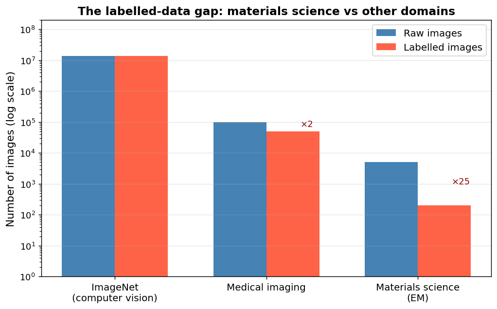
Labelled images per domain: ImageNet 14 M (crowdsourced, seconds each), medical imaging ~10⁴ (radiologists), materials EM 50–500 (hours of expert time each) Holm, Elizabeth A. et al., (2020); Sandfeld, Stefan et al., (2024).

• Walk through the three bars. Materials science sits three orders of magnitude below where ResNet-50 (25 million parameters) was designed to operate.
• The one point to land: the bottleneck is not pixels — a 4D-STEM dataset is hundreds of GB of raw frames. The bottleneck is expert annotation time. Raw data is abundant; labelled data is scarce.
• Why labels cost so much (formerly its own slide — say it, don’t show it): (1) acquisition cost — rationed beamtime, €3–8 M aberration-corrected TEMs; (2) expert annotation time — hours per SEM image, crystallographic expertise for HAADF defects; (3) reproducibility — a Zeiss and an FEI SEM give different contrast, so pooling silently introduces a domain shift (the Week 4 GroupKFold lesson at instrument level); (4) unique specimens — an AM turbine cross-section cannot be re-imaged. They compound.
• Rule of thumb: 50–500 labelled images per task; ResNet-50 at 500 images = 50 000 parameters per image.
• EM anchor: prior-β grain segmentation in titanium: half a day of preparation + one hour of annotation = one labelled image. EELS chemical-state labelling of a defect map takes hours per image.
• Transition: “The consequence for a naive deep-learning approach: overfitting.”

Overfitting at \(N\approx 50\): the model learns shortcuts

• ResNet-50 on 50 images: ~500 000 parameters per image — enough to fit any labelling, including noise.
• What it memorises instead of microstructure: detector vignetting, session contrast, the scale-bar corner.
• Symptom: a train–val gap (99 % train, 55 % test), not a high training loss.
• Diagnose: Grad-CAM (Week 7) lighting up corners or the scale bar; specimen-grouped validation.
• Hygiene rule: split by specimen first, then augment — the training set only.

• The shortcut-learning framing: the model is not “confused” — it correctly learns the most predictive feature in the training set, which happens to be a spurious correlation.
• The training/validation loss curve (backup slide “Small data → fast overfitting”) shows the classic picture: training loss falls monotonically, validation loss turns upward around epoch 40.
• Misconception to preempt: “I can fix overfitting by training longer.” No — longer makes it worse. The fixes are more labels, augmentation, transfer, synthetic or self-supervised pretraining: today’s topic.
• EM war story: a weld-defect classifier hit 99 % training / 58 % test. Grad-CAM showed it had learned the SEM vignetting pattern that correlated with the imaging session of the good welds. Fix: brightness augmentation + grouped cross-validation.
• Split-first, augment-second: with five specimens × 10 crops, a random 40/10 crop split puts every specimen on both sides and the model learns specimen identity. Right: 3 specimens / 2 specimens, then augment the 30 training crops. Group-based splits give lower and noisier numbers — that honest number beats a leaked one.
• Transition: “Four strategies attack this problem.”

The small-data survival kit: four strategies

1. Augmentation: physically plausible transforms multiply the effective training set.
2. Transfer learning: start from a pretrained backbone (ImageNet); adapt only the last layers.
3. Synthetic data: simulate images from known structures — perfect labels at zero annotation cost.
4. Self-supervised pretraining / foundation models: learn from unlabelled in-domain images, or start from DINOv2 / SAM.

• They stack: pretrained backbone → augmentation throughout → fine-tune on few real labels.

• Frame the four as independent angles: augmentation makes the most of the data you have; transfer imports features learned elsewhere; synthetic data provides free labels; self-supervision extracts features from unlabelled in-domain data. Together they can reduce the real label count from 500 to 20–50.
• The one point to land: “which one is best” is the wrong question. The exam expects the stacked pipeline, not a menu pick.
• Transition: “Start with augmentation — the cheapest lever.”

Augmentation: encoding physical invariances

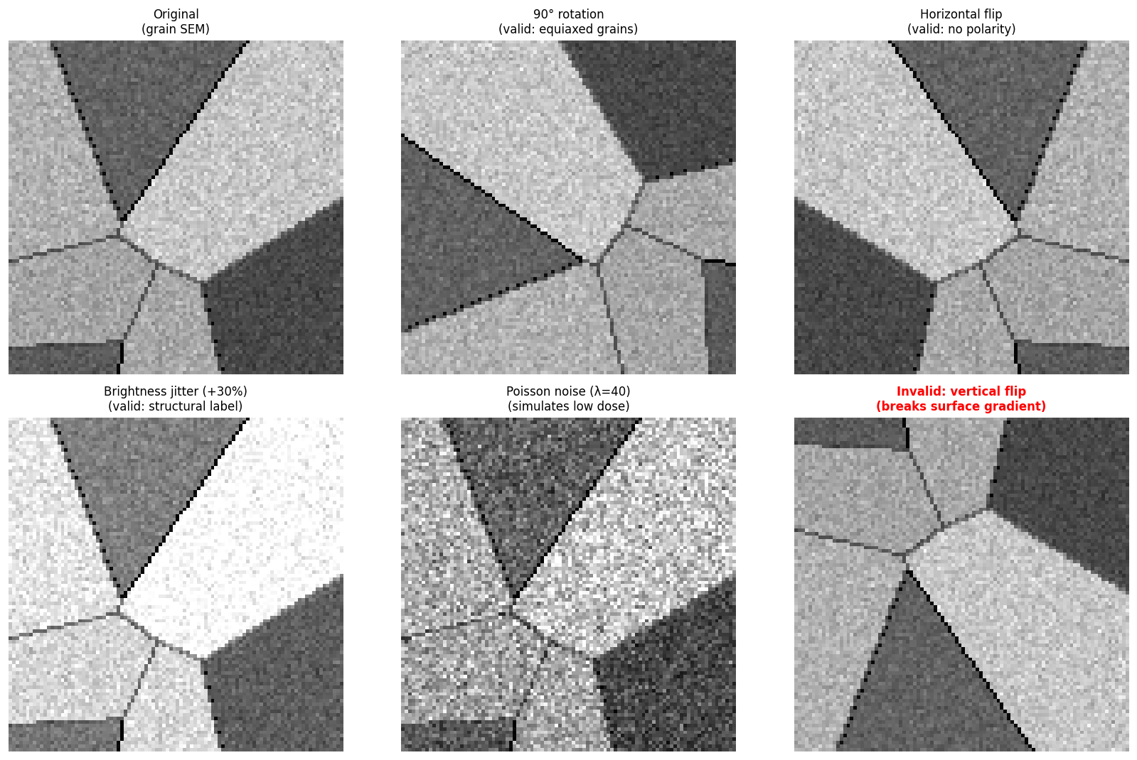
Six views of the SAME synthetic grain layout: original, 90° rotation, horizontal flip, brightness jitter, Poisson noise (all valid for equiaxed grains) and vertical flip (invalid if a surface gradient exists).

Every augmentation is a claim that the physics has that symmetry.

• Augmentation is not just multiplying data — it encodes a claim that the physics has a particular invariance. A rotation augmentation says “a grain boundary looks the same at any angle.” True for equiaxed grains; false for directionally solidified columnar grains, where orientation is a physical signal.
• The one point to land: “before adding any transform, ask: would this produce a physically plausible image with the same label? If not, it is label noise you injected by hand.”
• Misconception to preempt: “more augmentation is always safer.” Wrong. A wrong augmentation injects false invariances. Ablate augmentations one at a time if performance is unexpectedly poor.
• Transition: “What each transform encodes, and when it breaks.”

What each transform encodes — and when it is illegal

Transform	Physical claim / simulates	Illegal when …
Flip	mirror symmetry	feature has polarity (weld cap vs root, DS column)
Rotation	rotational symmetry	orientation is the signal (columnar grains, EBSD)
Crop / zoom	translation / scale invariance	grain size or lattice spacing is the label
Elastic warp	drift, sample warping	metric labels (size, aspect ratio)
Brightness / gamma	session / detector variation	intensity is quantitative (EELS, Z-contrast)
Poisson noise, blur	low dose, defocus, drift	rarely — the physically correct noise model
Scratches, contamination	preparation artefacts	artefact is the target

• Geometric transforms are claims about symmetries; intensity transforms are generally safer but the physics gate still applies when the label is intensity-calibrated.
• Poisson noise is the materials-literate distinction: generic CV adds Gaussian noise; in EM the correct noise is Poisson — signal-dependent, worst at low dose. A model augmented with realistic Poisson noise transfers to low-dose acquisition. Gaussian noise simulates readout noise and is also fine for structural labels.
• Blur forces the model to rely on topology rather than fine texture — exactly why synthetic grain detectors transfer.
• Synthetic scratches / contamination spots are the fix for last week’s scratch false positive: show the network artefacts during training so it learns they are not particles.
• Elastic warp on a grain-size regression task: the labels now refer to distorted grains. Symptom: worse on real images than the training curves predict.
• EM anchor for intensity: a carbon-contamination detector trained with brightness jitter ignores the subtle intensity change that is the only signal of contamination onset.
• Transition: “Three illegal cases you will meet in practice.”

Physically-invalid augmentations: the materials gate

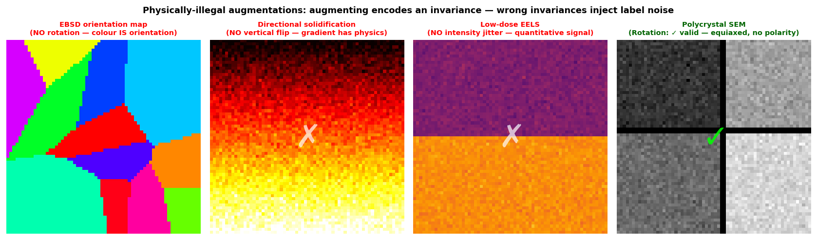
Illegal augmentations: rotating an EBSD/IPF map (colour encodes orientation), vertically flipping directional solidification (the thermal gradient is real), intensity jitter on an EELS map (intensity encodes composition). An equiaxed polycrystal allows all of them.

• This is the materials-specific key concept of the section — spend time here.
  1. EBSD rotation: the IPF colour IS the crystallographic orientation relative to the sample frame. Rotating the image without the colour key gives a pixel that says “30°” where the crystal is at “120°”. A labelling error with perfect data fidelity.
  2. Directional-solidification vertical flip: top and bottom of a DS column differ (segregation, dendrite morphology). A flip swaps them.
  3. EELS jitter: if the label is “42 % Fe”, ±20 % intensity jitter teaches a wrong intensity-to-composition map.
  4. Zoom/rescale when grain size or lattice spacing is the label (returns in SSL today).
• The one point to land: augmentation legality is a domain-knowledge decision. Ask a materials scientist, not a CV tutorial.
• Transition: “Apply the gate yourself — a cold-call scenario.”

Augmentation scenario: a laser-welded joint

• Scenario: 50 SEM images of a laser-welded joint, bead running left-to-right. Task: classify weld quality (good/defective).
• Horizontal flip: valid — the weld is approximately mirror-symmetric about its centreline.
• Vertical flip: invalid — top surface (cap bead, undercut) ≠ root (penetration, lack of fusion).
• 90° rotation: invalid — bead direction is physically defined (travel direction, gravity during solidification).
• Brightness jitter, Gaussian noise: valid — quality is a structural judgement, not an absolute-intensity measurement.
• The meta-point: every verdict came from physics, not from a CV default.

• Run as a cold-call: ask for each transform before revealing the verdict and the physical reason.
• A strong exam answer cites the physical reason, not just the verdict: “vertical flip is invalid because the cap differs from the root” passes; “vertical flip is invalid” does not.
• Misconception: “horizontal flip is always safe.” Only here because of the symmetry; the rule is task-dependent, not image-dependent.
• Transition: “Now the implementation: one transform for image and mask, and the split order.”

Implementation: joint transforms, on the fly, after the split

import albumentations as A
transform = A.Compose([A.HorizontalFlip(p=0.5), A.RandomRotate90(p=0.5),
                       A.GaussNoise(p=0.3), A.RandomBrightnessContrast(p=0.3)])
out = transform(image=image, mask=mask)   # ONE call: same random draw for both

• Label consistency: image and mask get the same sampled transform. Two separate calls → misaligned masks, IoU plateaus.
• On the fly: a new random transform every batch — the network never sees the same pixels twice.
• Split by specimen first, then augment the training set only.

• The classic bug: calling transform(image=img) and transform(image=mask) separately — two independent random angles. Symptom: training loss looks fine but IoU plateaus. The backup slide “On-the-fly augmentation and label consistency” shows the misaligned-mask picture.
• Each line of the config is a physics claim: HorizontalFlip claims mirror symmetry, RandomBrightnessContrast claims the label is structural. For the illegal cases two slides back (EBSD, directional solidification) you would remove HorizontalFlip / RandomRotate90.
• Offline augmentation (pre-generated on disk) gives a fixed set the network eventually memorises; use it only when the transform is expensive (e.g. physics rendering).
• Augmentation leakage: augmenting before splitting puts a rotated copy of a training image in the test set — the test then measures memorisation recall. Write “SPLIT, THEN AUGMENT” on the board.
• Transition: “Augmentation makes the most of the data we have. Transfer learning brings in knowledge from outside.”

Why ImageNet features transfer to EM images

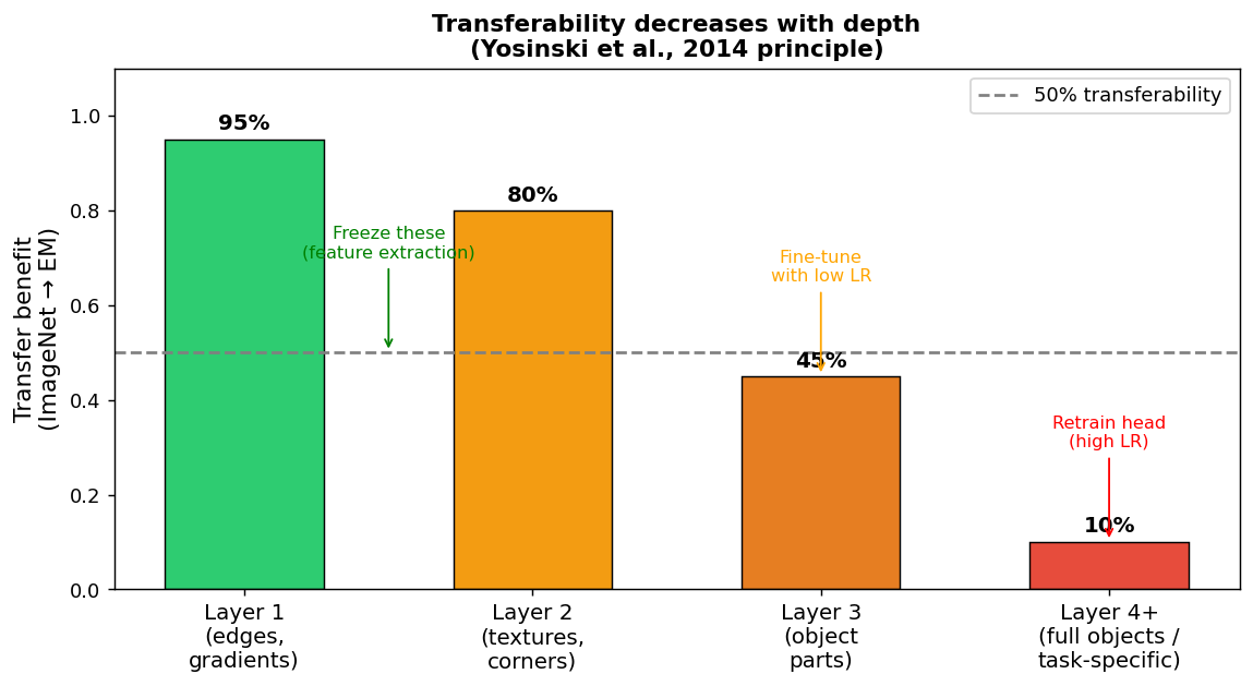
Transferability vs CNN depth Yosinski, Jason et al., (2014): edges/gradients (layer 1) transfer almost fully, textures mostly, object parts and task-specific layers barely.

• Domain gap: EM is 1-channel, 16-bit, Poisson noise, periodic textures. Replicate grey → 3 channels; do not re-initialise the first conv layer.

• Transferability decreases monotonically with depth. Early layers are constrained by natural-image statistics (edges, 1/f spectra) that EM images share; late layers are optimised for dogs, chairs and cars.
• Misconception: “ImageNet has no TEM images — how can it help?” Edge detectors fire at grain boundaries the same way they fire at the edge of a dog’s ear.
• The grayscale-to-RGB fix is the #1 silent bug. Re-initialising conv1 discards the most transferable layer. Correct: img.repeat(1, 3, 1, 1) or sum the pretrained RGB weights: w_gray = model.conv1.weight.sum(dim=1, keepdim=True).
• Texture mismatch (no Moiré fringes, lattice periodicity or diffraction banding in ImageNet) is what in-domain self-supervised pretraining closes later today.
• Actionable consequence: fine-tuning should be depth-graded — this is where differential LRs and gradual unfreezing come from.
• Transition: “The recipe: backbone plus head.”

Backbone + new head: feature extraction or fine-tuning?

	Few labels (<100)	More labels (100–1 000)
Small domain gap (optical ↔︎ photos)	Feature extraction (frozen backbone)	Fine-tuning, differential LRs
Large domain gap (photos ↔︎ HAADF)	Feature extraction + BN adaptation	Fine-tuning + gradual unfreezing

• Keep the backbone, replace the head — the 1000-class ImageNet head is discarded, never “fine-tuned”.
• BatchNorm trap: a frozen backbone in eval() uses ImageNet statistics → mis-normalised micrographs.

• Backbone = pretrained feature extractor (e.g. ResNet-50’s He, Kaiming et al., (2016) 2048-D representation). Head = randomly initialised task-specific map to your classes or scalar. Output dimension and semantics of the old head are both wrong.
• For segmentation the U-Net encoder IS the backbone; the decoder plays the role of the head.
• Zero real labels: synthetic pretraining → head, or synthetic pretraining → fine-tune.
• Feature extraction minimises overfitting risk but may underfit at a large domain gap; fine-tuning adapts features but risks catastrophic forgetting at small N.
• BN trap symptom: feature extraction is mysteriously poor. Fix: keep BN layers in train() mode (or re-estimate statistics) even when weights are frozen; typically recovers 5–15 percentage points.
• When in doubt, start with feature extraction; add fine-tuning once the head has converged.
• Transition: “Why fine-tuning needs different learning rates.”

Catastrophic forgetting and differential learning rates

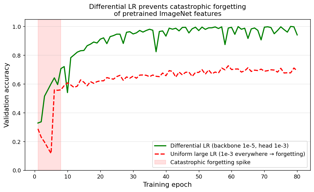
Fine-tuning with one large LR (red) destroys pretrained features in the first epochs; differential LRs (green) climb steadily.

• A random head sends large random gradients into the pretrained backbone and overwrites it.
• Fix: \(\eta_\text{backbone}\approx 10^{-5}\ll\eta_\text{head}\approx 10^{-3}\); unfreeze gradually top-down; or LP→FT.

• The mechanism is the exam concept: catastrophic forgetting is “a step size too large relative to the distance to a good minimum.” The backbone sits in a good basin; the head is far from any minimum.
• Recipe (backup slide “The transfer learning recipe”): stage 1 freeze everything, train the head at 1e-3; stage 2 unfreeze the last block at 1e-5; stage 3 continue unfreezing top-down with depth-graded LRs. Deepest (most task-specific) layers adapt first; earliest (most general) are preserved longest — the Yosinski curve made operational.
• LP→FT (later today): initialise the head from a linear probe so it never sends random gradients.
• Misconception: “just use one small LR for everything.” Then the head never learns. The fix is asymmetric rates.
• Symptom: loss spike at the start of fine-tuning, or final accuracy worse than feature extraction.
• Notebook: set backbone and head to the same LR and watch the spike; the fix is two parameter groups in Adam.
• Transition: “Transfer gives pretrained features. Synthetic data gives free labels.”

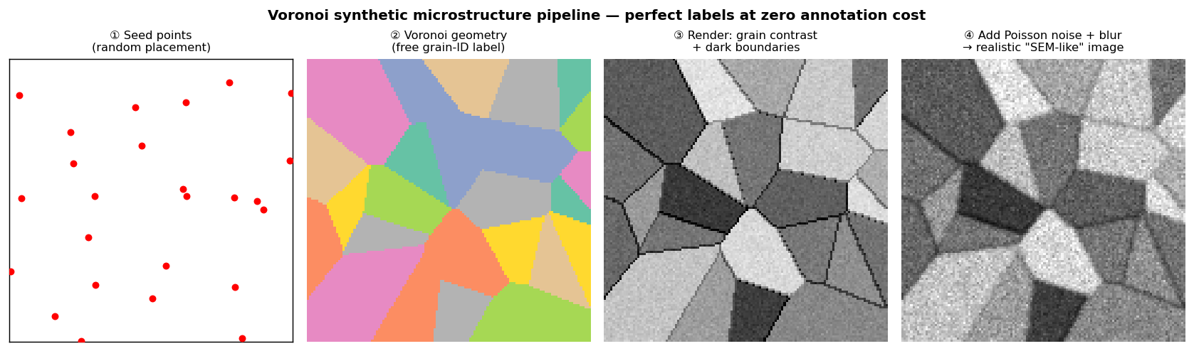
Synthetic data: free perfect labels by construction

• Flip the arrow: choose the label (structure) → render the image. The label is perfect by construction.
• Voronoi grains, phase field, multislice TEM Rakowski, Aaron et al., (2024): 10 000 images in minutes.
• Caution: it fails on whatever the generator omits — Voronoi makes no twins.

Voronoi pipeline: seeds → nearest-seed grain IDs (free labels) → per-grain intensity + boundaries → Poisson noise + blur.

• The labelling-arrow flip: standard annotation is image → label (human provides); synthetic is label → image (renderer provides). The label is an input, not an inference.
• Synthetic data converts the labelling problem into a modelling problem — the model is only as good as the generator’s physics.
• Walk the Voronoi panels: scatter seeds; assign each pixel to its nearest seed (grain ID known = free mask); random intensity per grain + dark boundaries; Poisson noise and defocus blur. A 30-line NumPy job; it is in the notebook.
• Caveat: Voronoi gives convex, roughly equiaxed grains with ~120° triple junctions — no annealing twins, no non-convex or columnar grains. The generator’s omissions become the model’s blind spots: not a tuning problem but an epistemic one.
• Transition: “Can purely synthetic training beat real labels? One case study.”

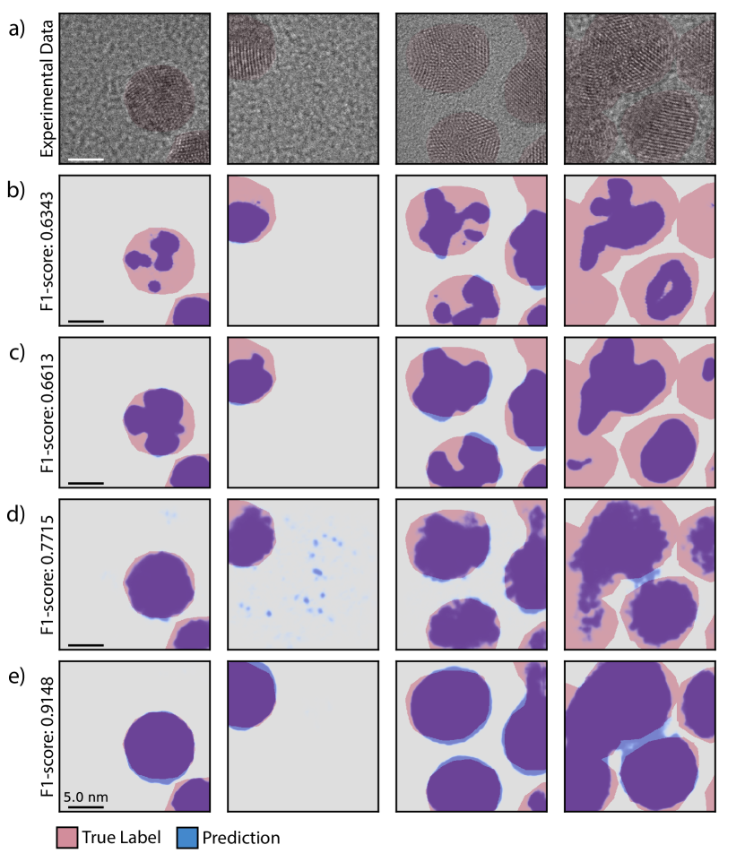
Purely synthetic can beat real-trained: Construction Zone

U-Net trained only on simulated HRTEM, tested on real nanoparticles Rakowski, Aaron et al., (2024):

Benchmark	Synthetic F1	Prev. best (real)
Au, 5 nm	0.92	0.89
Au, 2.2 nm	0.86	0.75
CdSe, 2 nm	0.75	0.59

Simulate the right variation, not more structures.

Synthetic-trained U-Net on real HRTEM Au nanoparticles; rows: weak → strong database curation. From Rakowski et al. 2024 Rakowski, Aaron et al., (2024).

• Construction Zone (Rakowski et al., npj Comput. Mater. 2024): random Au nanoparticles on carbon, multislice with thermal effects, aberrations, plasmon losses and Poisson dose noise → masks by construction. Zero experimental training images.
• Say the numbers, then the surprise: it beats models trained on annotated experimental data, especially in the data-scarce small-particle and CdSe cases.
• The twist: ablations showed a few atomic structures sufficed; what moved F1 was simulation fidelity (frozen phonons, residual aberrations, plasmons) and diversity of imaging conditions (defocus, dose, substrate thickness).
• This is the synthetic analogue of the augmentation lesson: the nuisance variation you inject makes the model robust. Our notebook uses the same idea (domain randomisation of blur and dose).
• Anti-pattern: a huge structure library at one defocus / one dose → perfect synthetic F1, collapse on real images. Diagnostic: hold out real images from epoch 0 and watch the gap.
• Transition: “When does synthetic transfer, and what do we do when it doesn’t?”

When synthetic transfers — and closing the sim-to-real gap

• It transfers when the generator captures the task-relevant invariant (grain topology: continuous boundaries, ~120° junctions) and spans the nuisance distribution (dose, defocus, aberrations).
• It fails on what the generator omits: twins, charging streaks, sub-grain contrast.
• Close the gap, boring solutions first:
  1. measured noise model (Poisson gain, readout σ) in the renderer
  2. augmentation in the rendering pipeline
  3. fine-tune on 10–20 real labels
  4. only then CycleGAN / adversarial domain adaptation

• Reconciliation of “synthetic fails on what the generator omits” and “a Voronoi-trained U-Net works on real SEM”: both are true. For grain-boundary detection the task reduces to “find the dark narrow strip between two regions”, which Voronoi captures. Grain size, triple-junction statistics, grain shape: work. Twin identification, specific texture components: do not.
• The sim-to-real figure (backup) shows clean synthetic vs real SEM with scan distortion, vignette and contrast drift — topology still correctly found.
• Failure scenario (backup): 96 % on synthetic, 61 % on real triple junctions — causes: geometry gap (rolled, elongated grains), missing artefacts (charging, contamination spots), contrast gap (channelling sub-structure), synthetic-style shortcut (Voronoi boundary width). “More synthetic data” does not help: more of a distribution that omits real artefacts still omits them.
• CycleGAN paints the real “texture skin” onto synthetic geometry while keeping the mask; adversarial DA makes features indistinguishable between domains. Both are unstable and only worth it with truly zero real labels.
• War story: a team spent a month on a CycleGAN; a colleague matched it in an afternoon by fitting a Poisson + Gaussian noise model to a flat-field image and fine-tuning on 20 real images.
• Transition: “Every fix so far needed labels or a physics generator. The fourth strategy needs neither.”

The unlabelled mountain: learning without labels

• Asymmetry: a 4D-STEM scan has \(10^5\)–\(10^6\) patterns; CEM500k holds ~500 000 unlabelled EM images Conrad, Ryan et al., (2021).
• Self-supervised learning (SSL): a pretext task whose labels come from the data itself trains a backbone; reuse it downstream.
• Goal: an embedding \(\mathbf{h}=f_\theta(\mathbf{x})\) where physically similar micrographs are close — so a few labels suffice.
• vs ImageNet transfer: SSL pretrains in-domain — your detector, noise and contrast.

• Classic pretext tasks: denoising (Week 9 autoencoders), predicting rotations, jigsaws, colourisation. Modern winners fall into three families: contrastive (SimCLR), masked modelling (MAE), self-distillation (DINO).
• SSL converts the labelling problem into a pretext-design problem. Pretraining and labelling are decoupled: pretrain once on everything, label a little per downstream task.
• Misconception: “self-supervised = unsupervised clustering.” No — SSL trains with a supervised-looking loss on manufactured labels. Clustering and latent spaces are next week.
• EM anchor: CEM500k (Conrad & Narayan 2021) — pretraining on a large unlabelled cellular-EM corpus gave better, more robust segmentation backbones than ImageNet.
• Transition: “The three families at a glance.”

Three families of self-supervised learning

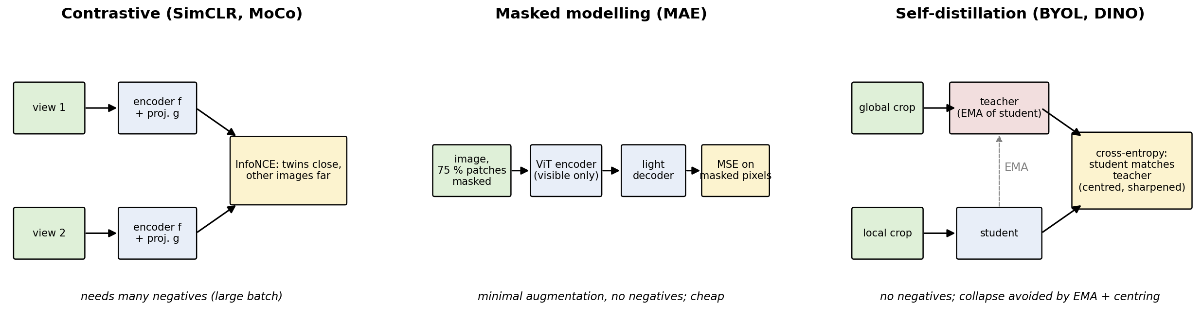
Contrastive: pull two views together, push other images apart. Masked modelling: hide patches, reconstruct them. Self-distillation: a student matches an EMA teacher across crops, no negatives.

Common enemy: representation collapse — every input mapped to the same vector.

• Walk left to right. Contrastive: “which of these is my twin?” Masked modelling: “fill in what is hidden.” Self-distillation: “agree with a slowly moving copy of yourself on a different crop.”
• Collapse trivially satisfies “views should agree”. Remedies: negatives (contrastive), a reconstruction target (MAE), EMA teacher + centring/sharpening (DINO).
• Transition: “Contrastive learning in detail — you implement it in the notebook.”

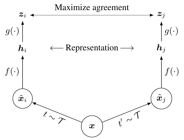
Contrastive learning: SimCLR

1. Batch of \(N\) micrographs, two random augmentations each → \(2N\) views.
2. Encoder \(f\) → \(\mathbf{h}\); projector MLP \(g\) → \(\mathbf{z}=g(\mathbf{h})\).
3. For view \(i\), its twin \(j\) is the positive; the other \(2N-2\) are negatives.
4. Minimise NT-Xent (InfoNCE); then discard \(g\), keep \(f\).

SimCLR: two augmentations of \(x\), shared encoder \(f\), projector \(g\). Only \(f\) is kept. Chen et al. 2020, Fig. 2 Chen, Ting et al., (2020).

• The projector matters: a loss directly on \(\mathbf{h}\) forces the encoder to discard everything the augmentations vary. With \(g\), the projector discards it while \(f\) keeps a richer representation — downstream tasks use \(\mathbf{h}\), not \(\mathbf{z}\).
• SimCLR needs many negatives: the original used batches of 4096. MoCo keeps a queue of negatives to decouple them from batch size.
• Notebook: batch 128, a 14 k-parameter CNN — enough to see the effect on CPU in about a minute.
• Transition: “The loss, written out.”

The InfoNCE / NT-Xent loss

For a positive pair \((i,j)\) among \(2N\) views, cosine similarity \(\mathrm{sim}(\mathbf{u},\mathbf{v})=\mathbf{u}^\top\mathbf{v}/(\|\mathbf{u}\|\|\mathbf{v}\|)\), temperature \(\tau\):

\[ \ell_{i,j} = -\log \frac{\exp\!\big(\mathrm{sim}(\mathbf{z}_i,\mathbf{z}_j)/\tau\big)}{\sum_{k\neq i}\exp\!\big(\mathrm{sim}(\mathbf{z}_i,\mathbf{z}_k)/\tau\big)} \]

• A \((2N-1)\)-way softmax classification whose “correct class” is the twin.
• Chance level \(\log(2N-1)\) (≈ 5.5 for \(N=128\)) — a sanity line on the training curve.
• Temperature \(\tau\) (0.1–0.5): small \(\tau\) focuses on the hardest negatives.
• Negatives prevent collapse: identical \(\mathbf{z}\) keep the loss at chance.

• Derive on the board: numerator = positive logit; denominator = positive plus all negatives. Exactly F.cross_entropy(sim / tau, target) with the diagonal masked — the 6-line implementation in the notebook. Same loss as Week 6 classification, with manufactured labels.
• Collapse: if all \(\mathbf{z}\) were identical, the denominator would be the numerator times \(2N-1\) — loss stuck at \(\log(2N-1)\).
• Large \(\tau\) treats all negatives alike; small \(\tau\) gives tight clusters but is less stable.
• Materials caveat: negatives are just other images in the batch. Two crops of the same specimen are false negatives and get pushed apart — sample batches across specimens.
• Transition: “The most important design decision is not the loss — it is the augmentation set.”

Augmentations are the labels: the physics gate returns

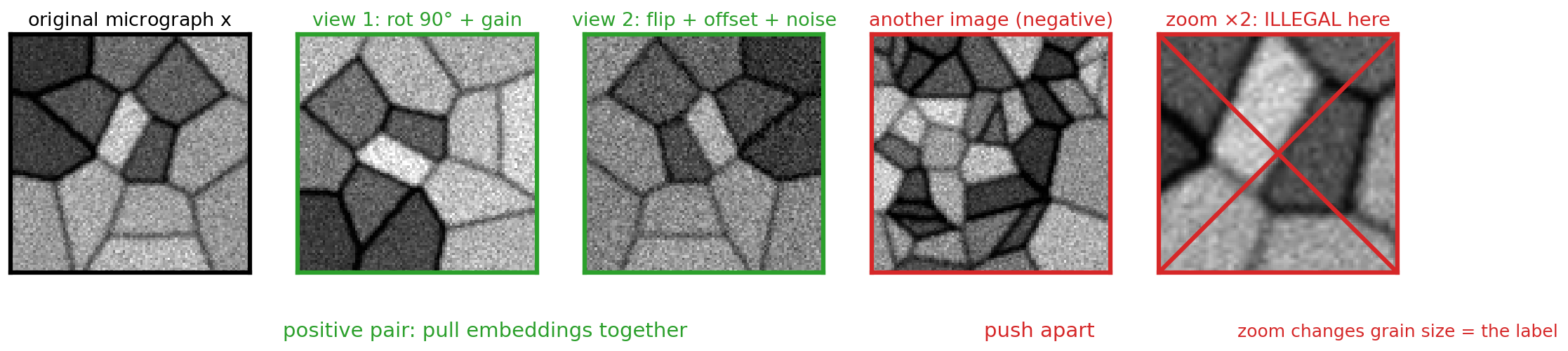
Rotation + gain and flip + offset + noise give a valid positive pair (green); another micrograph is a negative. A ×2 zoom is illegal when grain size is the target.

• The embedding becomes invariant to exactly the augmentations you use. Natural-image defaults (random-resized crop, colour jitter) are often wrong for EM.

• In SSL the augmentations are the only supervision. A wrong augmentation in supervised training adds label noise; a wrong augmentation in SSL deletes the information from the representation.
• Scale is physical (grain size, lattice spacing), intensity can be quantitative (Z-contrast, EELS), orientation can be the label (EBSD, texture).
• The zoom example is a notebook “try this yourself”: add a random zoom to SimCLR and watch the linear-probe accuracy for grain-size classes drop.
• EM anchors: 4D-STEM — rotations fine only if orientation does not matter; pattern-centre shifts (descan) are a nuisance and should be augmented. HAADF — a small lattice-spacing change is strain; scale augmentation erases it.
• Transition: “A different idea that needs almost no augmentation design: masking.”

Masked image modelling: MAE

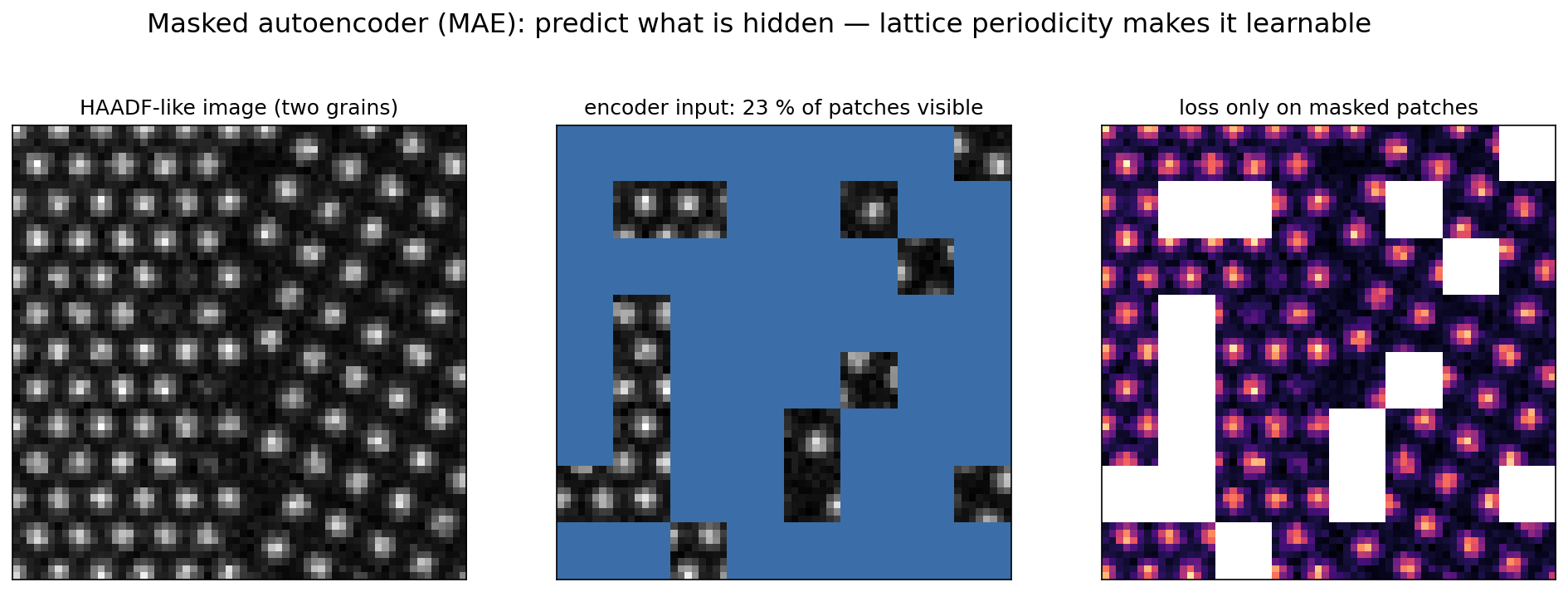
• Mask ~75 % of patches, encode the visible 25 % with a ViT, reconstruct the rest; MSE on masked patches He, Kaiming et al., (2022).
• High ratio → the model must learn structure, not interpolate.
• No negatives, minimal augmentation; encoder skips masked tokens (cheap).
• Frozen features weaker; MAE shines after fine-tuning.

MAE input for a HAADF-like two-grain lattice: 23 % of patches visible; the loss is on the hidden ones.

• MAE is the vision analogue of BERT; patches are tokens (transformers in Week 10). About 3–4× faster pretraining because masked tokens are never encoded.
• Why it suits EM: crystalline images are redundant — predicting a hidden patch requires knowing the lattice, its orientation and the grain boundary. Defects are where prediction fails, so masked-reconstruction error doubles as an anomaly detector.
• MAE features encode low-level pixel detail: a linear probe underperforms contrastive/DINO, but after fine-tuning MAE is among the best. Matters when choosing a protocol later.
• Collapse is avoided by the reconstruction target itself.
• Transition: “The third family drops negatives and reconstruction.”

Self-distillation: DINO and DINOv2

• Student–teacher: different crops (global + local); the student matches the teacher’s output distribution Caron, Mathilde et al., (2021).
• Teacher = EMA of the student — no gradients, a stable target (from BYOL Grill, Jean-Bastien et al., (2020)).
• No negatives: collapse avoided by centring and sharpening of teacher outputs.
• DINOv2 Oquab, Maxime et al., (2023): + masked-token objective, 142 M curated images. Frozen DINOv2 + linear probe = strongest generic baseline.

• Two networks agreeing with each other could trivially output a constant. Centring (subtract a running mean) prevents one dimension dominating; sharpening (low teacher temperature) prevents the uniform distribution.
• Local-to-global crops teach that a small patch “belongs” to the whole — DINO ViT attention maps segment objects without labels.
• For EM: DINOv2 backbones are the default starting point for “embed my micrograph archive”; ML-PC Unit 10 fine-tunes a DINOv2 ViT for in-situ AM quality control.
• Caution: multi-crop contains a scale assumption — the zoom problem again for grain-size tasks.
• Transition: “Side by side.”

SimCLR vs MAE vs DINO — what to use for EM?

	SimCLR	MAE	DINO / DINOv2
Signal	twin among negatives	reconstruct hidden patches	match EMA teacher
Collapse prevention	negatives	reconstruction target	EMA + centring + sharpening
Augmentation design	critical	minimal	important (multi-crop)
Frozen features	good	weaker	best
After fine-tuning	good	very good	very good

• Rule of thumb for 2026: (1) try frozen DINOv2 features first; (2) for modalities far from natural images (diffraction, spectra) with a large unlabelled corpus, pretrain in-domain with MAE (cheap: the encoder sees 25 %); (3) use SimCLR when you can articulate the invariances precisely and want a small CNN (needs large batches).
• I-JEPA (predict features of masked regions) is the direction the field is moving.
• Transition: “Has any of this been done on EM data?”

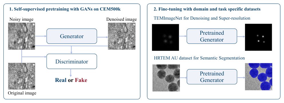
Self-supervised pretraining on EM data

• Kazimi et al. 2024 Kazimi, Bashir et al., (2024): pretrain on unlabelled CEM500k, fine-tune for segmentation, denoising, super-resolution.
• Smaller pretrained models beat larger random-init ones; biggest gains with few labels.
• Take-away: pretrain on the unlabelled mountain you already have.

Self-supervised pretraining on CEM500k, then fine-tuning on task data. From Kazimi, Ruzaeva & Sandfeld 2024 Kazimi, Bashir et al., (2024).

• The pretext here is adversarial denoising (a generator denoises, a discriminator judges real vs fake) — neither SimCLR nor MAE. The family matters less than the principle: in-domain pretraining on unlabelled EM data. CEM500k itself showed in-domain SSL beats ImageNet on EM segmentation benchmarks.
• “Smaller pretrained beats larger random”: at small N, initialisation, not capacity, is the bottleneck — the empirical version of today’s overfitting argument.
• Honest caveat: most published EM-SSL work is on biological EM. Materials-EM corpora of comparable size are only now appearing — an open opportunity for MSc/PhD projects.
• Transition: “Scale this up and you get foundation models.”

Foundation models: pretrain once, adapt everywhere

• Definition: a large model pretrained on broad data, adapted by prompting, probing or fine-tuning — DINOv2, CLIP Radford, Alec et al., (2021), SAM.
• Adaptation ladder: zero-shot / prompt → frozen features + probe / kNN → fine-tune last blocks → full fine-tune.
• For EM: natural-image models know edges, not diffraction physics — zero-shot is often mediocre; light in-domain fine-tuning closes most of the gap.

• CLIP: image–text embeddings, zero-shot classification by text prompts. SAM: promptable segmentation.
• Paradigm shift: instead of a model per task from scratch, start from a foundation backbone and spend the labelling budget on adaptation. Frozen features need one forward pass per image — laptop-feasible.
• “Foundation model” is not a quality guarantee; its fit to your modality must be measured (linear probe, retrieval — later today).
• Transition: “The foundation model most relevant to microscopists: Segment Anything.”

Segment Anything (SAM): promptable segmentation

• SAM Kirillov, Alexander et al., (2023): heavy ViT encoder (once per image) + prompt encoder + light mask decoder (per click, milliseconds).
• Promptable: click a particle or box a grain → mask; trained on 11 M images, 1.1 B masks.
• Zero-shot on EM: fine for particles and voids; weak on thin boundaries, low-dose noise, lattices.
• Real value: an annotation accelerator — clicks instead of polygons, then train your own small model.

• The encoder is MAE-pretrained; SA-1B was collected with a model-in-the-loop data engine. “Segment everything” mode tiles point prompts over the image.
• The encoder/decoder split is what makes interactive use feasible.
• Connect to active learning: SAM turns an hour of polygon annotation into a few minutes of clicking and correcting — it changes the cost side of the labelling equation.
• Misconception: “SAM understands microscopy.” It segments things that look like objects in natural photos; a low-contrast grain-boundary network or an atom-column lattice is not object-like.
• Transition: “What happens when you fine-tune it on microscopy?”

μSAM: Segment Anything for Microscopy

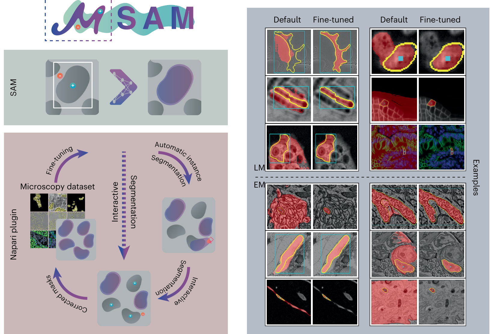
μSAM: napari plugin for interactive and automatic segmentation, correction and fine-tuning; default vs microscopy-fine-tuned results for light (top) and electron (bottom) micrographs. Archit et al., Nature Methods Archit, Anwai et al., (2025), doi:10.1038/s41592-024-02580-4.

Report zero-shot and fine-tuned results side by side.

• μSAM fine-tunes SAM on diverse light and electron microscopy data and ships generalist EM/LM models plus a napari tool for the annotate → correct → fine-tune loop.
• Finding: zero-shot SAM is mediocre on EM; fine-tuned generalist models are clearly better and cut annotation time; fine-tuning further on your own data helps again.
• Anti-pattern: never report zero-shot SAM numbers as “the method’s” performance, nor fine-tuned numbers without the zero-shot baseline.
• Materials note: published EM models are mostly biological EM. For nanoparticles or grains, expect to fine-tune on a few of your own images — today’s small-data setting.
• Transition: “Whatever backbone you choose — SimCLR, DINOv2, μSAM encoder — how do you use and evaluate its embeddings?”

Linear probe vs fine-tune vs from scratch

Protocol	What is trained	Use when
Linear probe (LP)	logistic regression on frozen \(\mathbf{h}\)	very few labels (≲ 50); measuring embedding quality
Fine-tune (FT)	backbone (small \(\eta\)) + head	more labels, larger domain gap
LP → FT	head from LP, then FT with small \(\eta\)	default fine-tuning recipe
From scratch	everything, random init	many labels, no relevant backbone

• The probe is a classifier and a measurement: is the information linearly present?
• LP→FT avoids random-head gradients distorting the backbone Kumar, Ananya et al., (2022). State protocol and \(N\); compare to random init.

• This is transfer learning revisited in embedding language: feature extraction = linear probe; fine-tuning with differential LRs = FT; gradual unfreezing and LP→FT answer the same catastrophic-forgetting problem.
• kNN on embeddings trains nothing — used for retrieval and sanity checks (next slides).
• Kumar et al. (ICLR 2022): full fine-tuning can underperform linear probing out of distribution because it distorts features; LP-FT gets the best of both. For EM, “out of distribution” = the next specimen, session or microscope.
• Always report “85 % (LP-FT, N = 300, grouped split)”. A number without protocol is uninterpretable, and without a random-init baseline you don’t know what pretraining bought.
• Transition: “What this looks like in the notebook.”

Notebook result: label efficiency of the protocols

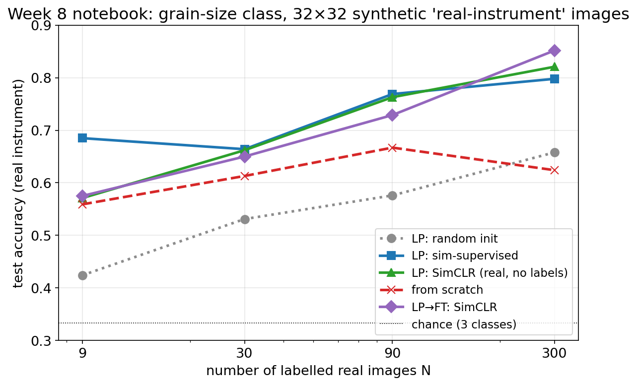
Test accuracy vs number of labelled “real-instrument” images, 3-class grain-size task: linear probes on random-init, sim-supervised and SimCLR backbones, plus LP→FT. From notebooks/week08_embeddings_transfer.ipynb.

• Setup: 32×32 synthetic micrographs, 2 random draws per N; SimCLR trained on 1 500 unlabelled “real” images; plot by img/make_figures.py.
• Read the curves: at N = 9 the sim-supervised probe (0.68) beats from scratch (0.56) — the simulator task needs exactly the feature the real task needs. From scratch plateaus around 0.6–0.67. LP→FT gains nothing over its probe at N = 9 (0.58 vs 0.57) but is best at N = 300 (0.85).
• SimCLR never saw a label yet overtakes the sim-supervised probe at N = 300 (0.82 vs 0.80).
• Random-init probe above chance: conv + pooling is itself an inductive bias.
• Honesty note: tiny task, two draws per N — trends, not benchmarks.
• Transition: “The second use of embeddings: retrieval — and checking the embedding before trusting it.”

Embedding retrieval and diagnostics

• Retrieval: L2-normalise \(\mathbf{h}_n\), rank by cosine similarity, score with precision@k. Notebook, \(k=5\) (chance 0.33): random 0.51 · SimCLR 0.67 · sim-supervised 0.72.
• Uses: find similar micrographs · de-duplicate before splitting · pick diverse images to label · flag OOD frames.
• Diagnose: linear probe vs random-init; inspect neighbours; colour the 2-D map by nuisance (session, detector).
• A pretty 2-D map is not evidence — trust the probe.

• Recipe: embed the archive once; for a query return the top-\(k\) by \(\hat{\mathbf{h}}_q^\top\hat{\mathbf{h}}_n\) (exact for 10⁵ images; approximate nearest-neighbour indices beyond). Precision@k = fraction of the \(k\) neighbours sharing the query’s label.
• What “similar” means is set by the pretraining: SimCLR with rotation augmentation retrieves grains at any orientation; an ImageNet embedding may retrieve by brightness or scale bar.
• Leakage use: near-duplicate crops of one specimen in train and test inflate every metric (Week 4); nearest-neighbour search finds them. OOD use previews Week 11: distance to the nearest training embedding is a simple OOD score.
• Colour-by-nuisance is the embedding version of Week 7’s shortcut demo: if points cluster by session, the embedding encodes the instrument, not the material. “Pretty t-SNE, dead downstream” — Week 9 covers how latent maps mislead.
• The random-init baseline: a random CNN already gets 0.51 precision@5 — only the improvement over that is due to pretraining. Also compare against hand-crafted Week 5 descriptors.
• When foundation embeddings fail: diffraction patterns, spectra, atom-resolved lattices; labels defined by a scale or intensity the pretraining made invariant → pretrain in-domain or fine-tune.
• Transition: “One more lever — spend the labels you do buy wisely.”

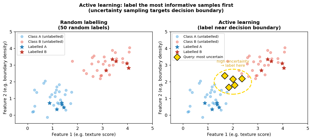
Active learning: label the most informative samples

1. Seed with 10–20 random labels (cold start).
2. Score all unlabelled images by uncertainty.
3. Query the most uncertain and diverse ones.
4. Retrain, repeat.

Random (left) vs active (right) labelling: the same 50 labels, concentrated near the decision boundary.

• Active learning fits when labels, not images, are the bottleneck — exactly materials EM.
• Uncertainty sampling: highest entropy / smallest margin. Diversity sampling: points unlike the labelled set. Best practice combines both.
• Cold-start warning: with no labels, uncertainty is meaningless — seed randomly first. Batch-diversity trap: pure uncertainty in batches picks a tight cluster of near-identical hard cases.
• 50 well-chosen labels can beat 500 random ones — not guaranteed; a high-leverage tool, not a free lunch.
• EM anchor: 500 diffraction patterns from an automated TEM session, budget for 30 expert labels: run the model, label the 30 least confident, retrain, repeat. Combined with SAM-assisted annotation, clicks replace polygons.
• The full workflow diagram is on a backup slide.
• Transition: “Put it all together.”

Putting it all together: 30 labelled TEM frames, 5 000 unlabelled

0. Split first by specimen/session; de-duplicate with retrieval.
1. Backbone: frozen DINOv2 / μSAM encoder, SSL on the 5 000 frames, or synthetic pretraining.
2. Diagnose: neighbours, precision@k, nuisance-coloured map; probe vs random init.
3. Adapt: linear probe first; LP→FT with differential LRs only if it beats the probe. Augment with the physics gate.
4. Spend labels wisely: SAM-assisted annotation + active learning; repeat 3–4.
5. Report honestly: held-out specimens, protocol and \(N\) stated.

• This is the synthesis of the lecture — every step maps to a section of today.
• The U-Net and CNN architectures from Week 7 are unchanged. What changed is how we initialise and train them.
• Validation hygiene overrides everything: a perfect pipeline with a leaky split produces a confidently wrong model. GroupKFold by specimen is the difference between a publishable number and a lie.
• Miniproject template: students with their own EM data should follow exactly these steps.
• Transition: “The notebook.”

Self-study notebook

notebooks/week08_embeddings_transfer.ipynb

1. Three data roles: labelled simulator, unlabelled “real” pool, few real labels + test set
2. Backbone A: supervised on the Voronoi simulator
3. Backbone B: SimCLR from scratch — NT-Xent in 6 lines, no zoom
4. PCA maps + kNN retrieval, precision@k
5. Scratch vs linear probe vs LP→FT for N = 9…300

Open in Colab

• CPU only, a few minutes.
• Try: zoom augmentation in SimCLR; naive FT vs LP→FT.

• Numbers: precision@5 random 0.51 · SimCLR 0.67 · sim 0.72; at N = 300 scratch 0.62 · SimCLR probe 0.82 · LP→FT 0.85. Optional section 6: frozen ImageNet ResNet-18 features (off by default). No downloads.
• Stress the zoom “try this yourself”: students see with their own eyes that the wrong augmentation deletes the information they need.
• The label-efficiency plot comes from this notebook (same code and seed); img/make_figures.py redraws it.
• Transition: “Summary.”

Summary: the week in six points

1. Labels, not pixels, are the bottleneck; at \(N\approx 50\) networks memorise shortcuts — grouped validation, split first.
2. Augmentation encodes physical invariances; illegal transforms inject label noise or erase the signal.
3. Transfer = backbone + new head; differential LRs, gradual unfreezing or LP→FT against catastrophic forgetting.
4. Synthetic data transfers when the generator captures the task invariant and spans the nuisance variation.
5. SSL pretrains on the unlabelled mountain (SimCLR, MAE, DINO); foundation models (DINOv2, SAM/μSAM) need in-domain adaptation.
6. Evaluate embeddings with probe, precision@k and nuisance-coloured maps, against random init.

• Read out loud; ask students to name, for each point, the slide or notebook cell that demonstrated it.
• Illegal examples to recall: EBSD rotation, DS flip, EELS intensity, zoom for size tasks. SimCLR = InfoNCE, augmentations are the labels; MAE = mask 75 %, reconstruct; DINO = EMA teacher, no negatives.
• Transition: “The must-know list for the exam.”

Must-know for the exam

• \(N\approx 50\) + \(10^7\) parameters overfits; train–val gap, Grad-CAM; split by specimen first, then augment.
• Augmentation legality: justify by physical symmetry; name an illegal case and why.
• Feature extraction vs fine-tuning (labels × domain gap); \(\eta_\text{backbone}\ll\eta_\text{head}\); catastrophic forgetting.
• InfoNCE: positives, negatives, temperature, chance level \(\log(2N-1)\).
• Collapse remedies: negatives (SimCLR), reconstruction (MAE), EMA + centring/sharpening (DINO).
• Linear probe vs LP→FT vs scratch; kNN retrieval with cosine similarity and precision@k.

• These mirror the written must-know list for Week 8 in the course exam document. The InfoNCE formula is on the InfoNCE slide: \(\ell_{i,j}=-\log\frac{\exp(\mathrm{sim}(\mathbf{z}_i,\mathbf{z}_j)/\tau)}{\sum_{k\neq i}\exp(\mathrm{sim}(\mathbf{z}_i,\mathbf{z}_k)/\tau)}\).
• Also on the written list: synthetic data transfer conditions, SAM/μSAM zero-shot vs fine-tuned reporting, embedding retrieval uses.
• Typical exam questions: design the augmentation set for a given EM task and justify it; write the InfoNCE loss and explain \(\tau\); interpret a label-efficiency plot; explain why zero-shot SAM numbers on EM data are not the method’s performance.

Next week: unsupervised learning, autoencoders & latent spaces

• Today: representations for a downstream label. Next: structure when there is no label — phases in a spectrum image, patterns in 4D-STEM.
• Clustering: k-means and Gaussian mixtures (EM algorithm).
• Autoencoders & VAEs: the reconstruction family — denoising AEs, ELBO, reparameterisation, rVAE.
• Latent maps and how they mislead: t-SNE/UMAP — today’s “pretty map” warning, made precise.

• Close the loop: MAE from today is an autoencoder with masking; next week starts from plain autoencoders and adds the probabilistic view (VAE).
• The one point to land: an embedding is only as meaningful as the objective that shaped it — next week, embeddings shaped by reconstruction and likelihood instead of downstream labels.
• Transition to the notebook: “Work through the notebook before Week 9 — especially the zoom-augmentation experiment.”

Continue

• ← Previous: Unit 07 — CNNs & U-Nets for microscopy
• → Next: Unit 09 — Unsupervised learning, autoencoders & latent spaces
• All courses

Backup slides

Material cut from the lecture path for time — for questions and self-study.

Small data → fast overfitting

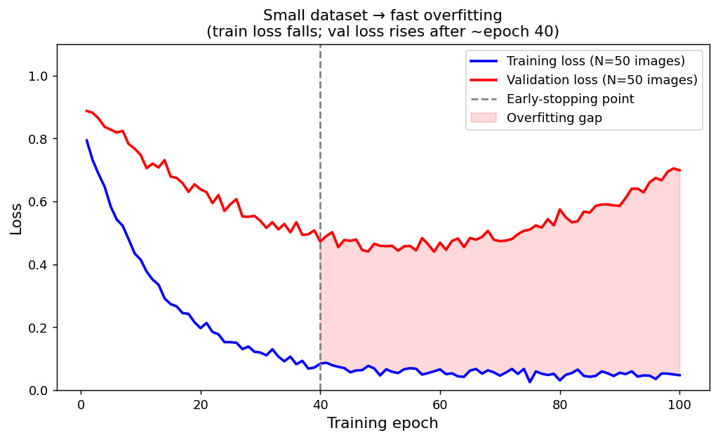
Training and validation loss for a CNN trained from scratch on 50 EM images. Training loss falls monotonically; validation loss starts rising around epoch 40 — the model is memorising the training images, not learning to generalise. The gap is the overfitting region.

• Walk through the two curves: the model memorises 50 images in 40 epochs; validation loss then diverges as it fits per-image noise — detector vignetting, brightness drift, instrument-specific contrast.
• The symptom is the train–val gap, not training loss. Training longer makes it worse.

On-the-fly augmentation and label consistency

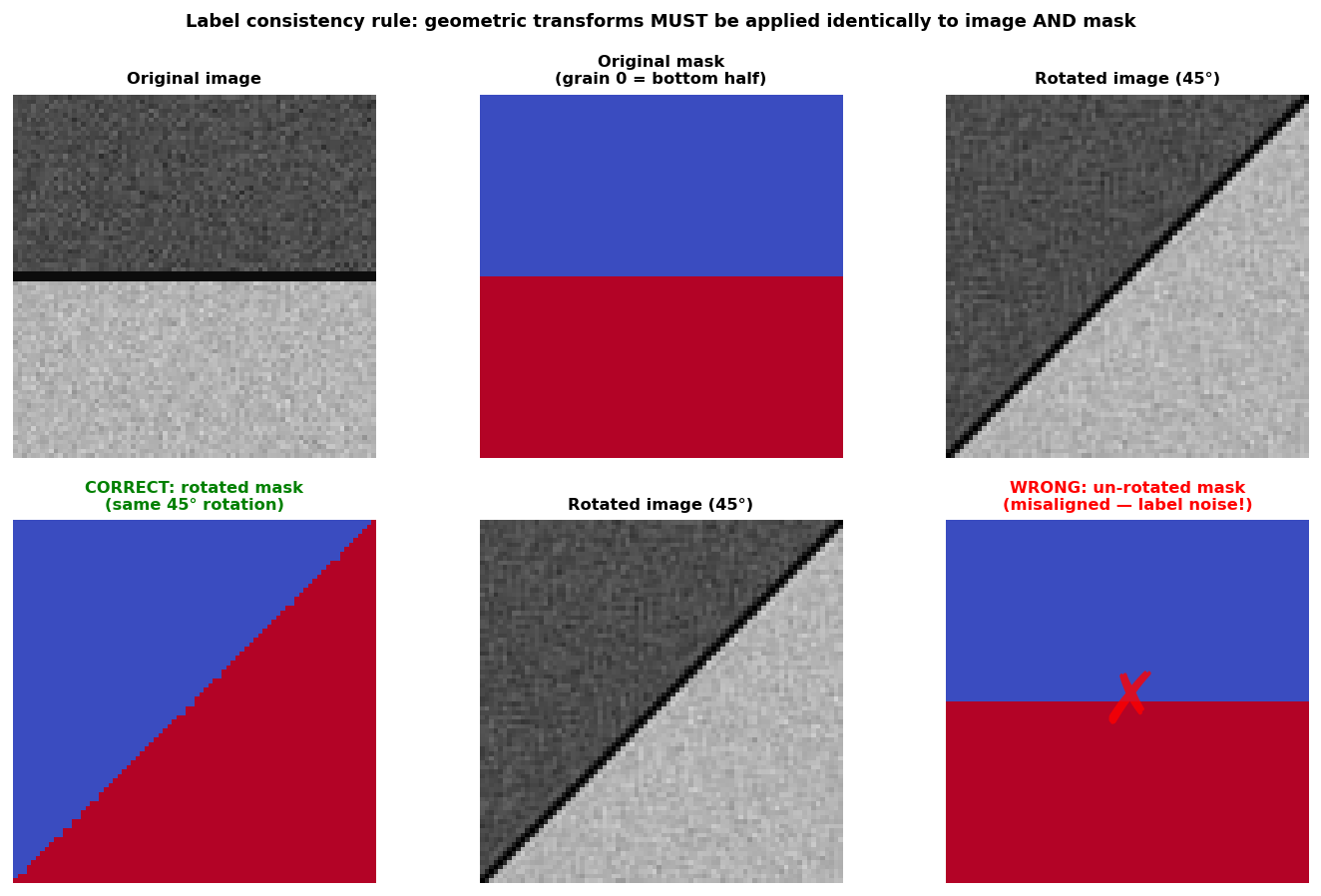
Label consistency: when a grain-boundary image is rotated 45°, the segmentation mask must be rotated by exactly the same 45°. Top row: original image, original mask, rotated image. Bottom row: correct — rotated mask (joint transform); wrong — un-rotated mask paired with the rotated image, producing misaligned ground truth.

• On-the-fly: a new random transform per batch — near-infinite effective dataset from 50 images. Offline: a fixed augmented set the network eventually memorises; only for expensive transforms.
• Split by specimen first, then augment the training set only.

The transfer learning recipe: freeze → head → fine-tune

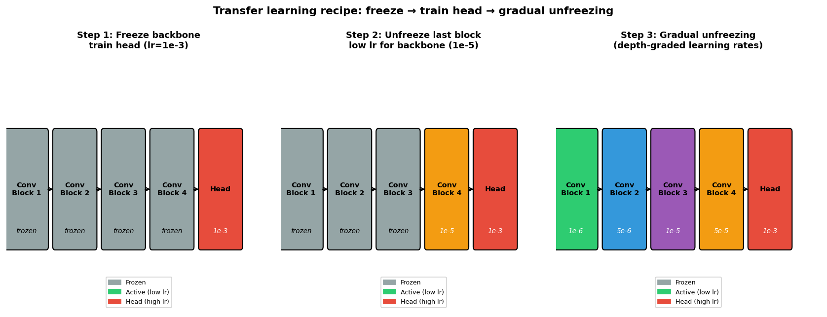
Three-stage transfer learning recipe. Stage 1: all backbone blocks frozen (grey); only the head (red) is trained at lr=1e-3. Stage 2: last backbone block unfrozen (orange) with low lr=1e-5; head continues at 1e-3. Stage 3: gradual unfreezing, depth-graded learning rates — early layers receive the smallest lr, late layers more, head the most.

• Head first, then top block, then deeper: the Yosinski depth curve made operational. Deepest layers are most domain-specific and adapt first; earliest layers are most general and are preserved longest.

The sim-to-real gap

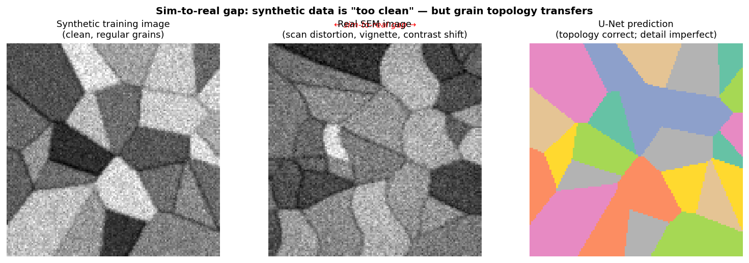
Three panels showing the sim-to-real challenge. Left: synthetic training image (clean, regular grains, no scan artefacts). Centre: real SEM image with scan distortion, vignette, and contrast drift relative to the synthetic distribution. Right: U-Net prediction — grain topology is correctly identified despite the gap, because topology is the task-relevant invariant.

• The gap is statistical: contrast, noise, spatial-frequency content and scan artefacts differ between generator and instrument. For grain topology the prediction survives; for anything more subtle expect the gap to hurt.

The sim-to-real gap: a failure scenario

• Scenario: a CNN trained on Voronoi images to detect grain triple junctions: 96 % on held-out synthetic data, 61 % on real SEM.
• Differential diagnosis:
  1. Geometry gap: rolled, elongated real grains vs convex equiaxed Voronoi grains.
  2. Missing artefacts: charging streaks, contamination spots that look like triple junctions.
  3. Contrast gap: real grains have sub-grain channelling contrast.
  4. Synthetic-style shortcut: the model learned Voronoi boundary-width regularities.
• The fix is not “more synthetic data” — add realistic rendering + fine-tune on 10–20 real images.

• Distinguish causes experimentally: test on an equiaxed real subset (geometry); mask or simulate artefacts; add grain-interior texture; Grad-CAM for the boundary-width shortcut.
• Callback to Week 4 leakage: the same failure mode (a spurious, perfectly predictive training feature) in a new context.

The complete small-data EM workflow

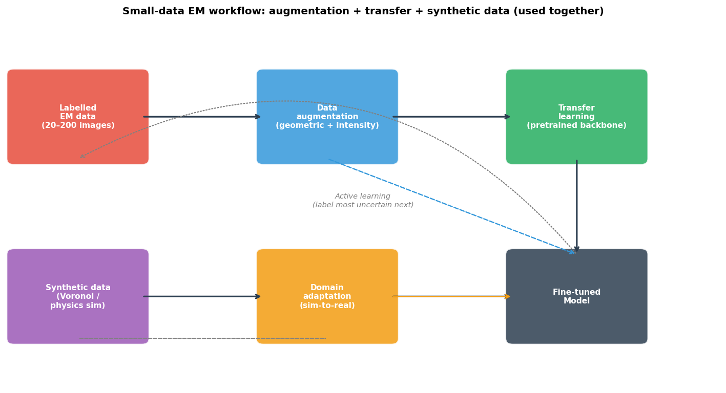
Complete small-data EM workflow diagram. The labelled EM data (20–200 images) feeds augmentation and transfer learning in parallel; synthetic data feeds domain adaptation; all three converge on a fine-tuned model. The active learning loop (dotted arrow, bottom) queries the fine-tuned model for the most uncertain unlabelled images, sends them to expert annotation, and grows the labelled pool.

• Self-supervised pretraining plugs into the transfer leg: it replaces the ImageNet backbone by one pretrained on your own unlabelled micrographs.

Validation in the small-data regime

• Group by specimen, not by crop: otherwise the model memorises specimen identity (vignette, brightness baseline, session contrast).
• Protocol: GroupKFold(n_splits=5).split(X, y, groups=specimen_ids) — the Week 4 lesson.
• Augmentation leakage: augmenting before splitting puts rotated copies of training images in the test set. Split first, then augment.
• Honest consequence: grouped splits give lower and noisier numbers — with 5 specimens the test set is 2 specimens. The variance is information.

• With only 50 images, one leaked specimen can inflate accuracy by 15–20 percentage points.

References

Overview: Computer vision and machine learning for microstructural characterization and analysis, Metallurgical and Materials Transactions A, Elizabeth A. Holm & others.

Materials data science, Stefan Sandfeld & others.

How transferable are features in deep neural networks?, Advances in neural information processing systems, Jason Yosinski, Jeff Clune, Yoshua Bengio, & Hod Lipson.

Deep residual learning for image recognition, Proceedings of the IEEE conference on computer vision and pattern recognition, Kaiming He, Xiangyu Zhang, Shaoqing Ren, & Jian Sun.

Construction zone: A machine learning dataset and benchmark for training and evaluating HRTEM nanoparticle segmentation algorithms, npj Computational Materials, Aaron Rakowski & others.

CEM500K, a large-scale heterogeneous unlabeled cellular electron microscopy image dataset for deep learning, eLife, Ryan Conrad & Kedar Narayan.

A simple framework for contrastive learning of visual representations, International conference on machine learning (ICML), Ting Chen, Simon Kornblith, Mohammad Norouzi, & Geoffrey Hinton.

Masked autoencoders are scalable vision learners, Computer vision and pattern recognition (CVPR), Kaiming He, Xinlei Chen, Saining Xie, Yanghao Li, Piotr Dollár, & Ross Girshick.

Emerging properties in self-supervised vision transformers, IEEE/CVF international conference on computer vision (ICCV), Mathilde Caron, Hugo Touvron, Ishan Misra, Hervé Jégou, Julien Mairal, Piotr Bojanowski, & Armand Joulin.

Bootstrap your own latent: A new approach to self-supervised learning, Advances in neural information processing systems (NeurIPS), Jean-Bastien Grill, Florian Strub, Florent Altché, Corentin Tallec, Pierre H. Richemond, & others.

DINOv2: Learning robust visual features without supervision, arXiv preprint arXiv:2304.07193, Maxime Oquab, Timothée Darcet, Théo Moutakanni, Huy Vo, Marc Szafraniec, Vasil Khalidov, Pierre Fernandez, Daniel Haziza, Francisco Massa, Alaaeldin El-Nouby, & others.

Self-supervised learning in electron microscopy: Towards a foundation model for advanced image analysis, arXiv preprint arXiv:2402.18286, Bashir Kazimi, Karina Ruzaeva, & Stefan Sandfeld.

Learning transferable visual models from natural language supervision, International conference on machine learning (ICML), Alec Radford, Jong Wook Kim, Chris Hallacy, Aditya Ramesh, Gabriel Goh, Sandhini Agarwal, Girish Sastry, Amanda Askell, Pamela Mishkin, Jack Clark, & others.

Segment anything, IEEE/CVF international conference on computer vision (ICCV), Alexander Kirillov, Eric Mintun, Nikhila Ravi, Hanzi Mao, Chloe Rolland, Laura Gustafson, Tete Xiao, Spencer Whitehead, Alexander C. Berg, Wan-Yen Lo, Piotr Dollár, & Ross Girshick.

Segment anything for microscopy, Nature Methods, Anwai Archit, Luca Freckmann, Sushmita Nair, Nabeel Khalid, Paul Hilt, Vikas Rajashekar, Marei Freitag, Carolin Teuber, Genevieve Buckley, Sebastian von Haaren, Sagnik Gupta, Andreas Dengel, Sheraz Ahmed, & Constantin Pape https://doi.org/10.1038/s41592-024-02580-4.

Fine-tuning can distort pretrained features and underperform out-of-distribution, International conference on learning representations (ICLR), Ananya Kumar, Aditi Raghunathan, Robbie Jones, Tengyu Ma, & Percy Liang.