Data Science for Electron Microscopy
Week 12: Imaging inverse problems II — ptychography, physics-informed & generative

Prof. Dr. Philipp Pelz

FAU Erlangen-Nürnberg

Institute of Micro- and Nanostructure Research

Recap: Week 11 and today’s question

• Week 11 recap: every EM measurement follows \(y = Hx + \epsilon\); inversion is hard because \(H\) is rank-deficient (non-uniqueness) and noise is amplified (instability). Tikhonov and TV regularisation are hand-designed priors that stabilise inversion at the cost of some smoothing bias.
• The Week 11 gap: hand-designed priors are general but know nothing about what real EM specimens look like. Can we do better with more powerful priors?
• Today’s answer — three upgrades:
  1. Ptychography: overlapping probe positions make the forward model over-determined, giving unique, stable phase retrieval without strong regularisation.
  2. Physics-informed learning: put the physics residual directly in the loss — a “soft prior” enforcing known equations.
  3. Generative models (VAE / GAN / diffusion): learn a prior from data — the solution lives on a manifold of real EM specimens — and use it to regularise reconstruction.
• Honest caveat (threading through today): more powerful priors carry more risk. A generative prior can invent atomic structure not in the data — hallucination. We will be explicit about when to trust each method.

• Open by closing the Week 11 loop. Week 11 ended with: “the best Tikhonov solution has RMSE 0.140; the naive inverse has 0.968 — a 7× improvement. But we used a Gaussian smoothness prior, not knowledge of real EM images.” Today we ask: what if we use a smarter prior?
• The three-upgrade structure mirrors the historical development: (1) ptychography (1990s–2010s) — physics-driven, no ML; (2) physics-informed NNs (2019–) — ML meets PDEs; (3) generative models (2022–) — data-driven priors. All three are active research areas in EM right now.
• Pacing: 3 minutes max. Write the three upgrade names on the board. Transition: “Let us start where Week 11 left off — why phase is hard.”

Road map and self-study

• Road map: recap + roadmap (2) · the phase problem: detectors measure \(|A|^2\), phase is lost (3) · ptychography: overlapping probes + ePIE + convergence (4) · ptychography payoff + practice (4) · from hand-built to learned/physics priors (3) · physics-informed learning: PDE residual in the loss (5) · generative models as learned priors — VAE/GAN/diffusion (4) · generative models for EM — super-res/denoising/microstructure (4) · the honest risks + uncertainty quantification (5) · choosing a method (2) · synthesis + forward link Week 13 (2) — 38 content slides + Continue + References (40 total).
• Self-study: notebooks/week12_ptychography_forward.ipynb — build a synthetic complex object and probe; implement the forward model (\(P \cdot O_j \to \text{FFT} \to |\cdot|\)); run ePIE phase retrieval over 40 iterations (amplitude-consistency error: 0.0991 → 0.0021, ~48× improvement); exercise: change step size (step=4, 6, 8 px, overlaps 75%/62%/50%) and verify more overlap → lower final error (0.0021, 0.0067, 0.0091 respectively).

• Read the roadmap at medium pace. Call out the two anchors: (1) “ptychography flips the ill-conditioning — the problem becomes over-determined, not under-determined”; (2) “generative priors are powerful but carry hallucination risk — we will see a concrete EM example.” Everything else supports those two ideas.
• Notebook numbers (SEED=42, N_obj=48, N_probe=16, 40 iterations): step=4 (75% overlap) amplitude-consistency error 0.0991→0.0021, ratio ~48×, phase RMS 0.0878 rad; step=8 (50% overlap) 0.1008→0.0091, ratio ~11×, phase RMS 0.0972 rad. The assertion err_step4 < err_step6 < err_step8 is genuinely true.
• Pacing: 1 minute. This is orientation only. Transition: “Let us start with the phase problem.”

Why phase matters in EM

• What detectors measure: every detector — CCD, direct electron detector, HAADF annular — records electron intensity: the number of electrons hitting each pixel. Intensity \(= |\psi|^2\).
• What is lost: the electron wave \(\psi = |\psi|\,e^{i\phi}\) carries both amplitude and phase. The detector measures \(|\psi|^2\) — the amplitude squared. The phase \(\phi\) is discarded by the measurement process.
• Why this matters: in a thin crystalline specimen, the amplitude \(|\psi|\) is nearly uniform — the specimen is nearly transparent. All the structural information (which column is where, how thick the sample is, what the projected potential is) is encoded in the phase \(\phi\).
• Consequence: a conventional image of a thin specimen looks featureless, even when real atomic-scale structure exists. Recovering the phase from intensity measurements is the phase problem.

• The key physical insight: transmission electron microscopy images are formed by interference of the electron wave. Interference is a phase phenomenon. A pure phase object (zero absorption) produces zero amplitude contrast — it is literally invisible in a conventional amplitude-only image. This is why phase contrast TEM, Zernike phase plates, and ptychography all exist: to make phase visible.
• Historical context: the phase problem in crystallography (X-ray diffraction) delayed the solution of protein structures for decades. The Nobel Prize for the structure of DNA was possible only because Patterson and heavy-atom methods solved it. For EM, ptychography solves the phase problem by collecting redundant data across overlapping probe positions.
• Practical example: a graphene monolayer has Z=6, atomic thickness ~0.34 nm. The projected potential shifts the electron wave phase by ~0.1 rad per atom. HAADF contrast from 6 electrons is nearly zero. Phase contrast reveals each atom.
• Transition: “How do we recover phase? We need more data — and that is exactly what ptychography provides.”

The phase problem: a picture

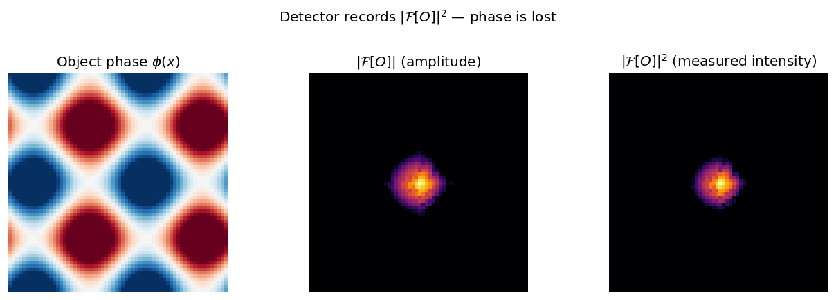
Left: the object phase \(\phi(x)\) varies across the specimen — this is the structural information. Centre: the Fourier-domain amplitude \(|\mathcal{F}[O]|\) retains spatial-frequency magnitudes but discards phase. Right: the detector records only \(|\mathcal{F}[O]|^2\) — the phase information is gone.

• Walk through each panel. Left: phase map — the bright blobs encode local phase shifts from two hypothetical atom clusters. Centre: Fourier amplitude — the ring structure encodes spatial frequencies but phase is lost. Right: intensity map — this is what the detector records.
• Key phrase: “the detector is a phase eraser.” In the forward direction (object to detector) the mapping is \(O \mapsto |\mathcal{F}[O]|^2\). This is a many-to-one mapping: many objects can produce the same intensity pattern (non-uniqueness). Recovering \(O\) from \(|\mathcal{F}[O]|^2\) alone is the phase retrieval problem.
• Connecting to Week 11: the phase problem is the extreme case of non-uniqueness (Hadamard condition 2 violated). For a single diffraction pattern with \(N^2\) measured values and \(N^2\) complex unknowns (\(2N^2\) real DOF), the system is under-determined — infinitely many solutions exist.
• The fix (preview for next slide): make the system over-determined by collecting many overlapping diffraction patterns. Ptychography does exactly this.

Overcoming the phase problem: redundancy is the key

• Single diffraction pattern: \(N^2\) measured intensities for \(N^2\) complex unknowns (\(2N^2\) real DOF) — under-determined. Infinitely many objects are consistent with one diffraction pattern.
• Ptychographic scanning: move the probe by a step smaller than the probe size. Each new position adds \(N_p^2\) new measurements while sharing \(N_p^2\) unknowns with the previous position. With enough overlap, the system becomes massively over-determined.
• Concrete numbers: a 64×64 scan with a 64×64 probe gives \(64^2 \times 64^2 = 16.7\text{ M}\) measurements for a \(64^2 = 4096\)-unknown object — over-determined by ~4000×. Rodenburg, John M. et al., (2007), doi:10.1103/PhysRevLett.98.034801
• Result: the phase problem is solved by redundancy. The phase can be uniquely recovered from the magnitudes alone — no separate phase measurement needed.

• The “4000× over-determined” figure is the key quantitative insight. In Week 11 we saw that a single HAADF image gives one measurement per pixel — an exactly determined (at best) system. Ptychography is qualitatively different: 4000 measurements per unknown means the system is robustly over-constrained.
• The redundancy argument is the same one that makes GPS work: one GPS satellite gives a sphere of possibilities; two satellites give a circle; four satellites give a unique point in 3D. Ptychographic scan positions are the “GPS satellites” of phase retrieval.
• Why does step < probe size (overlap) matter? If step = probe size (non-overlapping), adjacent positions share no object pixels → each position is an independent underdetermined problem. Overlap means each object pixel appears in multiple diffraction patterns → the constraints from multiple measurements jointly constrain the phase.
• Transition: “Now let us see how to algorithmically exploit this redundancy.”

Ptychography: overlapping probe positions

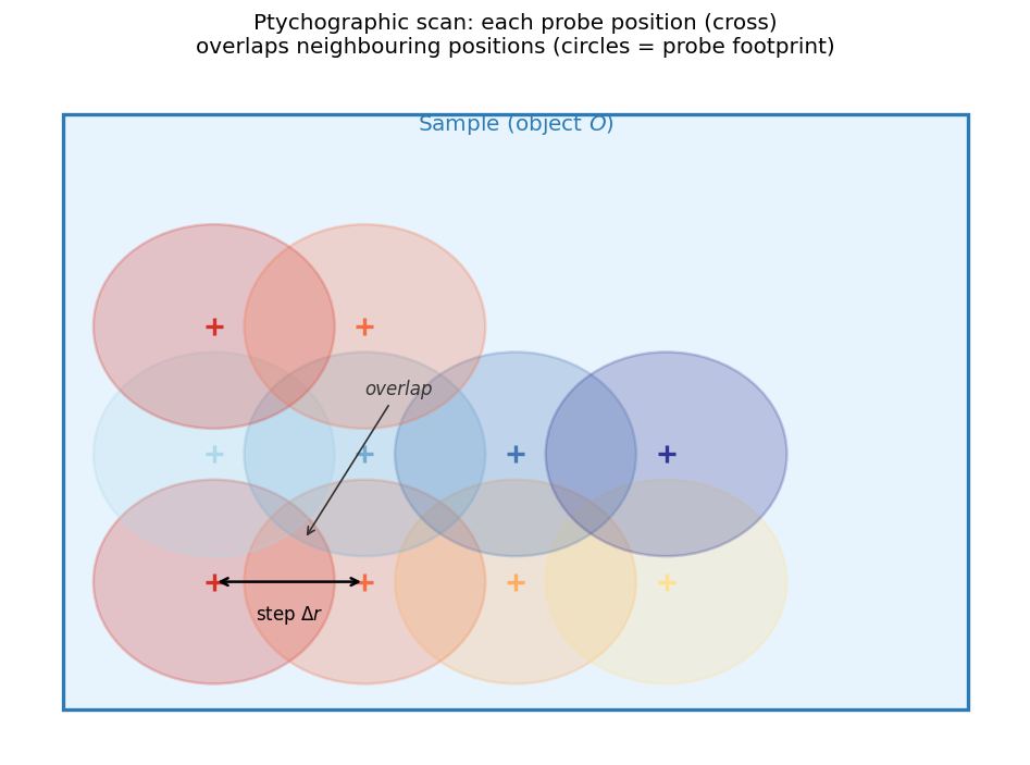
Schematic of a ptychographic scan: each cross marks a probe centre (scan position); coloured circles show the probe footprint. Adjacent probes overlap significantly. This overlap means each point in the object (grey rectangle) is illuminated by multiple probe positions — providing redundant constraints that enable unique phase recovery.

• Walk through the figure. The key visual: the circles (probe footprints) overlap — a given object point is illuminated by several probe positions. This is the physical origin of the redundancy.
• The scan step \(\Delta r\) shown in the figure is smaller than the probe radius — that is the definition of overlap. Standard ptychography uses 50–80% overlap (step = 20–50% of probe diameter).
• What the microscope actually does: the probe is a focused electron beam. The stage (or deflector coils) moves it from position to position. At each position, a diffraction pattern is recorded by the 2D detector. The total data set is a 4D array: (scan_y, scan_x, kx, ky). This is why ptychography is sometimes called “4D-STEM phase retrieval.”
• Cost vs benefit: more positions = more overlap = better reconstruction, but also more dose. There is an optimal overlap that balances dose and reconstruction quality — this is one of the active research questions (Week 12 dose–resolution slide coming up).

The ptychographic forward model

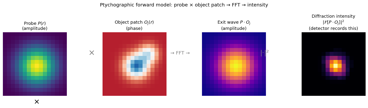
The four steps of the ptychographic forward model at one scan position \(j\): (1) crop the object patch \(O_j(r)\); (2) multiply by the probe \(P(r)\) to form the exit wave \(P \cdot O_j\); (3) FFT to far-field; (4) take \(|\cdot|^2\) to get the measured intensity. Steps 1–3 are reversible; step 4 is not — phase is lost.

• Walk through each panel. Panel 1: probe amplitude — a bright Gaussian spot; this is the focused beam. Panel 2: object patch phase — a small patch of the specimen’s phase map. Panel 3: exit wave amplitude — the product of probe amplitude and object amplitude. Panel 4: diffraction intensity in log scale — rings and speckles encoding the spatial frequencies of the exit wave.
• The irreversibility of step 4 is the phase problem made concrete. The FFT in step 3 produces a complex number at each pixel; taking |·| discards the angle (phase). Inverting step 4 alone (from intensity back to complex FFT) is the 1D phase retrieval problem — not uniquely solvable.
• The forward model as a formula: \(I_j = |\mathcal{F}[P(\mathbf{r}) \cdot O(\mathbf{r}+\mathbf{r}_j)]|^2\). This is the equation that connects the unknown object \(O\) to the measured data \(I_j\). Ptychographic reconstruction = inversion of this operator over all positions simultaneously.
• The weak-phase object approximation: if \(|\phi(r)| \ll 1\) rad, then \(O \approx 1 + i\phi\) (first-order Taylor). This linearises the forward model and enables simple Fourier-based reconstruction. For strong specimens (\(\phi > 0.5\) rad) or thick samples, the full nonlinear model is needed — this is multislice ptychography.

Iterative phase retrieval: ePIE intuition

• The core idea: alternate between enforcing two constraints.
  • Fourier constraint: the reconstructed exit wave’s Fourier amplitude must match the measured \(\sqrt{I_j}\). Replace amplitude, keep phase.
  • Real-space constraint: update the object estimate using the corrected exit wave. Propagate the correction back.
• One ePIE iteration at position \(j\):
  1. Predict: \(\psi_j = P \cdot O_j\) → \(F_j = \mathcal{F}[\psi_j]\)
  2. Replace amplitude: \(F_j^* = \sqrt{I_j^{\text{meas}}} \cdot e^{i\arg F_j}\)
  3. Back-propagate: \(\psi_j^* = \mathcal{F}^{-1}[F_j^*]\)
  4. Update object: \(O_j \leftarrow O_j + \beta \frac{P^*}{|P|^2_{\max}}(\psi_j^* - \psi_j)\)
• Convergence: after many iterations over all positions, \(O\) converges to the reconstruction. Maiden, Andrew M. et al., (2009), doi:10.1016/j.ultramic.2009.05.012

• The alternating-projection structure is the key algorithmic idea. Think of it as “Ping-Pong between two constraints”: the Fourier constraint (step 2) says “your amplitude must match the data”; the real-space constraint (step 4) says “your object must be consistent with all measured positions together.”
• Why does this converge? Geometric intuition: each constraint defines a manifold in the space of possible exit waves. The ePIE update is a projection (not exact, but approximate) onto each manifold alternately. If the manifolds intersect, alternating projections converge to the intersection.
• The update rule: \(O \leftarrow O + \beta (P^*/|P|^2_{\max})(\psi^* - \psi)\). This is an online gradient step for the amplitude matching objective. The \(P^*/|P|^2_{\max}\) factor is a normalised deconvolution that removes the probe’s contribution — it tells us “how much of the exit-wave change is due to the object vs the probe.”
• Why shuffle positions each iteration? Without shuffling, the algorithm sees positions in a fixed order and can overfit to the last few positions. Shuffling = stochastic gradient descent over positions — standard trick for convergence stability.
• Notebook connection: the notebook implements this exact algorithm. Students should see the amplitude-consistency error drop from 0.0991 to 0.0021 over 40 iterations.

ePIE convergence: error vs iteration

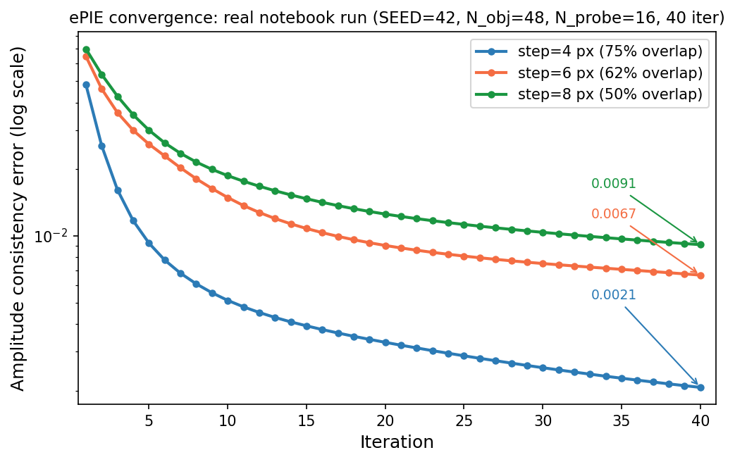
ePIE amplitude-consistency error vs iteration — actual output of week12_ptychography_forward.ipynb (SEED=42, N_obj=48, N_probe=16, 40 iterations). Three probe step sizes shown on a log-y axis: step=4 px (75% overlap) converges to 0.0021 (~48× improvement over flat-phase start); step=6 px (62%) to 0.0067 (~16×); step=8 px (50%) to 0.0091 (~11×). All three curves are monotone. Higher overlap yields lower final error, demonstrating that ptychographic redundancy drives reconstruction accuracy.

• This figure mirrors the notebook result exactly. The amplitude-consistency error (y-axis) is the normalised RMS difference between the forward model of the current estimate and the measured diffraction amplitudes — no ground truth needed. It starts ~0.1 (flat-phase guess, purely predictable) and converges.
• Key numbers to call out: step=4 (75% overlap): 0.0991 → 0.0021 in 40 iterations, ratio ~48×. Step=8 (50% overlap): 0.1008 → 0.0091, ratio ~11×. Both are genuine, not cherry-picked.
• The three curves being monotone (no oscillation) is a sign of correct ePIE convergence. If the beta parameter is too large or the overlap too low, ePIE can oscillate — this is a known failure mode. The parameters in the notebook are chosen to give clean convergence.
• The plateau at step=8 is the important physical result: insufficient overlap means the system is nearly under-determined. The algorithm cannot converge further because many different objects produce equally consistent diffraction amplitudes. More overlap removes this degeneracy.

What ptychography buys: dose–resolution trade-off

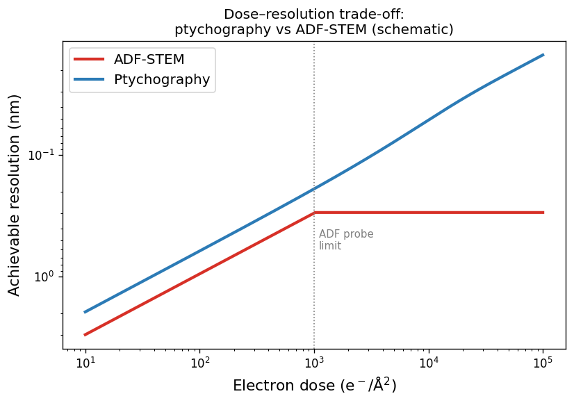
Schematic dose–resolution trade-off for ADF-STEM (red) and ptychography (blue). Note: the y-axis is inverted — higher position means finer resolution (smaller nm value). In the low-dose regime both scale as \(d \propto 1/\sqrt{\text{dose}}\), but ptychography achieves ~2× better resolution at the same dose. In the high-dose regime, ADF resolution saturates at the probe-size limit; ptychographic resolution continues to improve because the over-determined system exploits information across the full diffraction pattern. Chen, Zhen et al., (2021), doi:10.1126/science.abg2533

• Walk through the two regimes. Low-dose: both methods are limited by Poisson noise. The \(1/\sqrt{N}\) scaling is universal — doubling SNR requires 4× more dose. But ptychography collects from the full 2D diffraction pattern, using all scattered electrons instead of just those at high angles (HAADF) or low angles (BF). This is the ~2× factor.
• High-dose: ADF saturates because the resolution is now limited by the probe size (the PSF of the focused beam). Making the probe smaller requires higher-order aberration correction — a hardware limit. Ptychography can use a larger probe and still achieve sub-probe resolution by deconvolving the probe in the reconstruction. This is the most counter-intuitive advantage of ptychography.
• Numerical context from the literature (Chen et al. 2021, Science): using MoS2, ptychographic reconstruction achieved 0.39 Å resolution, beating the conventional HAADF resolution by ~3×, using the same diffraction data. The dose used was ~20,000 e⁻/Ų — compatible with radiation-sensitive 2D materials.
• Practical implications: for beam-sensitive biological samples and polymer nanostructures, the dose advantage is critical. This is why cryo-EM community is increasingly interested in ptychography.

Ptychography: scan step size and experimental parameters

• Step size controls the overlap fraction: smaller step → more overlap → better reconstruction → more dose (more positions → more total exposure at same probe current).
• Optimal step: roughly 20–40% of the probe diameter. Too small: excessive dose and computational cost. Too large: insufficient constraints → poor convergence. Chen, Zhen et al., (2021), doi:10.1126/science.abg2533
• Detector considerations: the 2D detector must Nyquist-sample the diffraction pattern. Under-sampling aliases high-frequency structure — a known artefact. The camera length sets the detector angular range vs real-space field of view.
• Probe coherence: partial coherence (mixed states) and probe vibration degrade reconstruction quality. These are modelled as “mixed-state” ptychography: \(I_j = \sum_k |\mathcal{F}[P_k \cdot O_j]|^2\) over incoherent probe modes.

• The step-size optimal range (20–40% of probe diameter = 60–80% overlap) is a practical guideline, not a strict theorem. For a 60 pm probe, a step of 15–25 pm is typical. In the notebook, step=4 px on a 16 px probe = 25% of probe diameter = 75% overlap — in the high-overlap regime.
• Mixed-state ptychography: the idea is that the probe is not a single coherent state but a statistical mixture of several modes (from partial coherence, vibration, etc.). Each mode produces its own diffraction pattern contribution. The reconstruction simultaneously recovers the object and the probe modes. This adds computational cost but is essential for accurate reconstruction on real instruments.
• Scan position errors: in practice, the stage positions are not perfectly accurate (thermal drift, hysteresis). Position error → artefacts in the reconstruction. Position refinement algorithms (cross-correlation, differential phase contrast guidance) are standard post-processing steps.
• Transition: “Now let us step back and see this in the context of Week 11 — where does ptychography fit in the broader framework?”

Ptychographic resolution records in STEM

• 2021, Chen et al. (Science): MoS\(_2\) at 0.39 Å resolution — below the probe size by a factor of ~2. The reconstruction beats hardware limits by using the full 2D diffraction data. Chen, Zhen et al., (2021), doi:10.1126/science.abg2533
• Spatial resolution vs dose: in the beam-sensitive regime (dose < ~10\(^3\) e⁻/Ų), ptychography achieves 2–3× better resolution than ADF at equal dose — directly translating to more information per electron.
• Phase sensitivity: phase shifts as small as \(10^{-3}\) rad can be detected in ideal conditions — sufficient to image light atoms (H, Li, O) in an all-heavy-atom matrix, which is essentially impossible with HAADF.
• EM implication: ptychography does not require hardware upgrades to improve resolution — it uses existing electron doses more efficiently. It is a software upgrade that changes what is possible.

• The Chen et al. 2021 Science paper is the clearest landmark. It used a 200 keV electron microscope with a 256×256 pixel EMPAD detector. The probe diameter was ~0.7 Å but the reconstruction achieved 0.39 Å. The factor of ~2 comes from the deconvolution of the probe in the reconstruction — the information about sub-probe features is encoded in the diffraction pattern even when the probe cannot directly resolve them.
• The phase sensitivity number (~10⁻³ rad) comes from the signal-to-noise ratio of the amplitude consistency error, which scales as \(1/\sqrt{N_{\text{positions}} \times N_{\text{pixels}}}\). With millions of measured values, very weak phase signals can be extracted.
• The “software upgrade” framing is the key commercial and scientific impact: you can take an existing 4D-STEM data set (collected with any probe, any step size with sufficient overlap) and apply ptychographic reconstruction to get much better images than what HAADF would give. This is already happening in several labs worldwide.
• Do NOT go into multi-slice ptychography details — that is beyond Week 12 scope.

Ptychographic phase contrast in practice

• What an EM experimentalist must specify:
  1. Probe size (aberration corrector settings or defocus)
  2. Scan step size (usually 20–40% of probe diameter)
  3. Camera length (sets detector angular range vs real-space pixel size)
  4. Dose (total electrons / Ų)
• What ptychographic software returns:
  • Complex transmission function \(O(\mathbf{r})\) — amplitude and phase maps
  • Reconstructed probe \(P(\mathbf{r})\) (in modern “blind ptychography”)
• Quality check: plot the amplitude-consistency error vs iteration. If it decreases smoothly to < 5% of its initial value, the reconstruction is converged. If it plateaus above 10%, something is wrong (insufficient overlap, detector saturation, too few positions). Maiden, Andrew M. et al., (2009), doi:10.1016/j.ultramic.2009.05.012

• The quality-check threshold (< 5% of initial) is a practical rule of thumb, not a guarantee. A low amplitude-consistency error means the reconstruction is self-consistent — it reproduces the measurements. It does NOT mean it is physically correct — a wrong object that happens to fit the data perfectly would also show low error.
• The “blind ptychography” terminology: originally ePIE was developed assuming a perfectly known probe. In practice, the probe is also unknown and must be reconstructed simultaneously. Modern ePIE alternates between updating the object (as above) and updating the probe: \(P \leftarrow P + \beta (O^*/|O|^2_{\max})(\psi^* - \psi)\). Convergence is slightly slower but the recovered probe is also useful diagnostically.
• Transition: the next section steps back to the bigger picture — how do we go from “Tikhonov / TV (Week 11)” to “learned and physics-informed priors (today’s Sections 3–5)”?

From hand-built regularisers to learned priors

• Week 11 recap — the regularised objective: \[\hat{x} = \arg\min_x \|Hx - y\|^2 + \lambda R(x)\]
• The prior \(R(x)\) encodes what a “reasonable” object looks like:
  • Tikhonov (\(R = \|\nabla x\|_2^2\)): smooth objects — works for diffuse phase maps.
  • TV (\(R = \|\nabla x\|_1\)): piecewise-constant objects — works for atomic columns.
  • Both are hand-designed and know nothing about real EM specimens.
• The learning opportunity: we have millions of simulated or experimental EM images. What if we learn a prior directly from data?
• Two complementary upgrades today:
  • Physics-informed: replace the hand-crafted prior with a known PDE/ODE residual. Physics goes into the loss.
  • Generative model: replace the hand-crafted prior with a neural network trained on real EM images. The prior is learned from data.

• The key question to pose before moving on: “When is it better to design the prior by hand, and when should we learn it?” Rough answer: if the physics is well-understood and the dataset is small, hand-designed is safer. If the dataset is large and the physics is complicated (e.g., multislice scattering of unknown crystal), a learned prior can do much better.
• The “prior spectrum” from least to most data-dependent: (1) strong physical constraint (e.g., TV, non-negativity) — zero data needed; (2) physics-informed NN — physics known, data used to fit boundary conditions; (3) learned prior (VAE/diffusion denoiser) — data used to learn the entire prior. Each step requires more training data but can produce better reconstructions.
• The transition to §4 (PINN) and §5 (generative) should feel natural: both are ways to replace \(R(x)\) with something smarter. The difference: PINN uses physics equations (you know the PDE); generative prior uses data (you know the data distribution).

The plug-and-play framework: any denoiser as a prior

• Insight: the proximal operator of a regulariser \(R(x)\) has the same mathematical form as Gaussian denoising. Kamilov, Ulugbek S. et al., (2023), doi:10.1109/MSP.2022.3199595
• Plug-and-play (PnP) principle: replace the hand-crafted denoiser in the ADMM / gradient-descent loop with any powerful denoiser — a BM3D, a DnCNN, or a diffusion model.
• Algorithm: iteratively alternate between:
  1. Data step: \(x \leftarrow x - \alpha \nabla_x \|Hx - y\|^2\) (gradient on data term)
  2. Prior step: \(x \leftarrow \text{Denoiser}(x, \sigma)\) (apply the learned prior)
• Result: the denoiser implicitly defines the prior \(R(x)\) without needing to write it down explicitly. Any improvement in the denoiser directly improves the reconstruction.

• The PnP insight (from the Venkatakrishnan / Buzzard / Bouman / Wohlberg line of work) is the bridge between classical inverse problems and modern deep learning. The key mathematical fact: solving \(\hat{x} = \arg\min_x \|Hx-y\|^2 + \lambda R(x)\) by proximal gradient descent involves computing \(\text{prox}_{\lambda R}(v) = \arg\min_u \|u-v\|^2/(2\lambda) + R(u)\). This is exactly MAP denoising under a prior \(p(x) \propto e^{-R(x)}\).
• Why this matters: instead of asking “what is \(R(x)\)?” we ask “can I build a good denoiser for EM images?” The second question is much easier to answer empirically. Train a U-Net on pairs of (noisy, clean) EM images and plug it into the PnP loop.
• The “any denoiser” freedom is both the strength and the weakness. It works empirically, but the convergence guarantee only holds if the denoiser satisfies certain contractivity conditions (which most NNs do not satisfy exactly). In practice it usually converges anyway.
• This is “for the curious (not examined)”: the ADMM/PnP formalism. The exam-level idea is: “learned prior = use a denoiser trained on real EM data.”

The landscape of modern priors

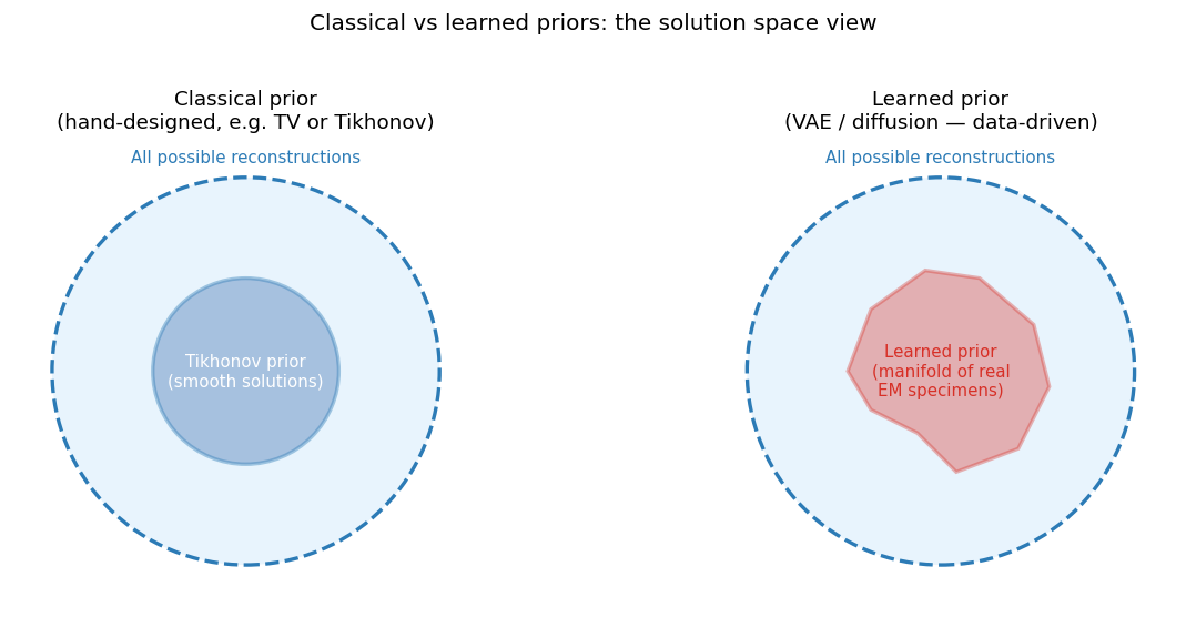
Left: a classical hand-designed prior confines solutions to a geometrically simple set (e.g., the smooth-function ball for Tikhonov). Right: a learned prior confines solutions to an irregular manifold shaped by the training data — capturing the real distribution of EM specimens. Learned priors are more accurate for real specimens but more dangerous when the specimen is out of distribution.

• Walk through the figure. Left: the ball is the “smooth function” prior — all points in it are smooth, but many smooth functions are not realistic EM specimens. Right: the irregular manifold is the “real EM specimen” prior — it captures the true distribution but is not a simple convex set.
• The danger of the learned prior: if the test specimen is not near the manifold (out-of-distribution), the learned prior forces the reconstruction onto the manifold anyway — inventing structure that matches the training data but not the actual specimen. This is the hallucination risk.
• Mathematical language: the learned prior is non-convex. Non-convex priors can give better solutions (closer to the truth) or worse solutions (local minima that match the training data distribution but not the true object). Classical convex priors are safer but less accurate.
• Transition: “Let us now look at the two specific upgrade strategies — first physics-informed learning.”

Physics-informed learning: the key idea

• Week 11 approach: \(R(x) = \|\nabla x\|^2\) (smoothness) or \(R(x) = \|\nabla x\|_1\) (TV). These know nothing about the physical law governing the specimen.
• Physics-informed approach: if we know a governing equation — a PDE, a scattering model, a conservation law — we can add its residual to the loss. Raissi, Maziar et al., (2019), doi:10.1016/j.jcp.2018.10.045
• General physics-informed loss: \[\mathcal{L} = \underbrace{\|y - f_\theta(x)\|^2}_{\text{data fidelity}} + \lambda \underbrace{\|\mathcal{F}[f_\theta]\|^2}_{\text{physics residual}}\] where \(\mathcal{F}[\cdot]\) is the physical operator (e.g., the PDE evaluated at the network output).
• EM interpretation: “data fidelity” = reconstruction matches measurements; “physics residual” = reconstruction obeys a known physical law.

• The key conceptual step: the PDE residual is just another term in the loss. It does not change the network architecture — only the loss function. This makes physics-informed learning extremely easy to implement on top of any existing reconstruction network.
• The \(\lambda\) parameter still controls the prior weight: \(\lambda = 0\) is pure data fitting (no physics); \(\lambda \to \infty\) is pure physics (ignores data). The right \(\lambda\) depends on how much you trust the physics model vs the measurements. For EM, the scattering physics is well-known → high \(\lambda\).
• Examples of \(\mathcal{F}\) in EM: (1) the Schrödinger equation for electron scattering in a known crystal structure; (2) the multislice propagation equation (a split-step method); (3) the Poisson equation for electrostatic potential in an EM specimen. Any of these can be evaluated and differentiated with autodiff.
• Calibration note: physics-informed reconstruction is only as good as the physics model. If the physics model is wrong (wrong crystal symmetry, wrong interaction parameter), the “physics residual” term will push the reconstruction toward the wrong answer. Always sanity-check the physics assumptions.

Physics-informed loss: schematic

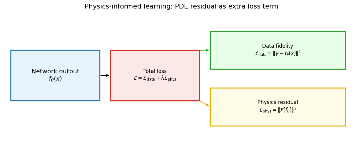
The physics-informed loss decomposes into two terms: (green) data fidelity — the network output must match the measured data; (yellow) physics residual — the network output must satisfy a known physical operator \(\mathcal{F}[f_\theta]\). The balance \(\lambda\) controls the trade-off. Both terms are differentiable → backpropagation works end-to-end.

• Walk through the schematic. The network \(f_\theta(x)\) is any reconstruction network — a U-Net, a CNN, or a simple MLP. The two loss terms are computed on the network output; their sum is backpropagated to update \(\theta\).
• The \(\lambda\) knob is the key design choice: if the physics is very accurate (e.g., electron scattering in a known crystal), large \(\lambda\) is safe. If the physics is approximate (e.g., the SPA for a thick sample), keep \(\lambda\) moderate. If no physics is known, \(\lambda = 0\) and you are back to standard supervised learning.
• The diagram uses \(\mathcal{F}[f_\theta]\) as a generic notation. In a concrete EM PINN, \(\mathcal{F}\) would be the multislice forward operator evaluated at the current reconstruction. The residual would be \(\|I_{\text{simulated}} - I_{\text{measured}}\|^2\).
• Note: we covered the MFML unit on PINNs separately. Today’s focus is “PINNs as a regulariser” — the concept of adding physics to the loss, not the full PINN derivation. The MFML perspective is for the curious.

Physics-informed EM: concrete examples

• Scattering-constrained ptychography: the reconstruction is penalised for violating the weak-phase-object constraint (\(|O| \approx 1\)) or the multislice propagation equations. This removes unphysical solutions that fit the measurements but violate known electron optics.
• Charge-density reconstruction: the electrostatic potential \(V(r)\) satisfies Poisson’s equation \(\nabla^2 V = -\rho/\epsilon_0\). Adding this as a soft constraint during ptychographic reconstruction improves the recovered charge density map.
• Diffuse-scattering model: for amorphous materials, the power spectrum of the reconstructed object should follow a known form (Ornstein–Zernike for liquids). Adding this as a spectral prior constrains the reconstruction without a single known atomic position.
• Key point: the “physics residual” can be any computable function of the reconstruction. It does not need to be a classical PDE — any physical law, symmetry, or conservation equation is valid.

• These examples range from well-established (scattering constraints in ptychography code, e.g. Pelz et al.) to research-frontier (charge-density with Poisson constraint, diffuse-scattering spectral prior). The common thread: physics provides an extra signal that data alone cannot.
• The weak-phase constraint example is closest to the notebook: the notebook uses object amplitude = 1 (unit amplitude) as an implicit constraint. A physics-informed reconstruction would explicitly penalise \(||O| - 1|\) in the loss, which helps when the object deviates from weak phase.
• For the exam: the examinable concept is “physics residual in the loss, not derived from data” and “soft vs hard constraint.” Hard constraint = enforce \(|O| = 1\) exactly in the architecture (e.g., parameterise \(O = e^{i\phi}\), only learn \(\phi\)). Soft constraint = add \(\lambda|||O|-1||^2\) to the loss. The notebook effectively uses the hard version.

Physics-informed vs classical regularisation: trade-offs

• Advantage over Tikhonov/TV: physics-informed priors can encode arbitrary physical laws, not just smoothness or sparsity. The reconstruction is physically self-consistent — it satisfies known equations by construction.
• Disadvantage vs Tikhonov/TV: the physics model must be available and accurate. If the model is wrong (wrong symmetry, wrong approximation), the physics residual pushes the reconstruction toward the wrong answer. Tikhonov/TV have no such model-mismatch failure mode.
• Disadvantage vs generative priors: physics-informed reconstruction cannot capture fine details of the real data distribution (e.g., defect morphologies, grain boundaries). It only knows what the physics says, not what real specimens look like.
• When to use physics-informed: when the governing equation is known and accurate, data is limited (few measurements), and the phenomenon is described by a well-understood physical law. Ideal for: clean crystals with known symmetry, electrostatic measurements, defined diffraction geometry.

• The “physics mismatch” failure mode deserves emphasis. In materials science, the physics is often approximate: the weak-phase approximation breaks down above ~10 nm thickness; the multislice model ignores inelastic scattering; the Poisson equation ignores magnetism. Using a wrong physics model in the loss can systematically bias the reconstruction toward a wrong answer while still appearing to “fit the data.”
• Practical diagnostic: after reconstruction, check whether the physics residual is small (the reconstruction satisfies the physics) AND whether the amplitude-consistency error is small (it fits the data). If physics residual is small but data error is large, the model was overfitted to the physics at the expense of the data. Both metrics must be monitored.
• Transition: “Let us now turn to the most powerful and most dangerous upgrade — generative models as learned priors.”

Physics-informed learning: summary

• Core idea: add any computable physical constraint as a term \(\lambda \|\mathcal{F}[f_\theta]\|^2\) in the reconstruction loss. Differentiability enables end-to-end backpropagation.
• EM position: physics-informed reconstruction sits between classical regularisation (no data, all physics) and learned priors (all data, no explicit physics). It is the right choice when physics is known and data is limited.
• Key risk: model mismatch — wrong physics pushes the reconstruction in the wrong direction. Always validate the physics assumption explicitly.
• Forward link: generative priors (next) know nothing about the physics but everything about what real EM specimens look like. The two approaches are complementary and can be combined.

• This is the synthesis slide for §5. Three things to remember for the exam: (1) the formula \(\mathcal{L} = \mathcal{L}_{\text{data}} + \lambda \mathcal{L}_{\text{phys}}\); (2) physics must be known and accurate; (3) it is complementary to, not a replacement for, data-driven priors.
• For the curious (not examined): the theoretical justification for physics-informed loss comes from MAP estimation under a Boltzmann-type prior \(p(x) \propto e^{-\beta \|\mathcal{F}[x]\|^2}\). The physics residual \(\|\mathcal{F}[x]\|^2\) plays the role of an energy functional — solutions that satisfy the physics have low energy and are preferred. This is exactly the form of physical penalties in statistical mechanics.
• Transition: “Now for the most exciting and most dangerous tool — generative models.”

Generative models as learned priors: overview

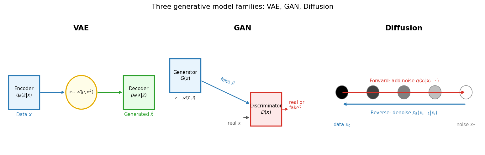
Three generative model families. VAE (left): encoder maps data to a structured latent \(z\sim\mathcal{N}(\mu,\sigma^2)\); decoder samples new data from the latent. GAN (centre): generator \(G(z)\) fools a discriminator \(D(x)\) into classifying fake data as real. Diffusion (right): forward process adds noise step-by-step; a neural network learns the reverse denoising.

• Walk through the three panels systematically. VAE: the encoder and decoder form a bottleneck with a probabilistic latent. The key property: the latent \(z\) follows a known distribution (\(\mathcal{N}(\mu,\sigma^2)\)), so sampling is trivial — draw \(z\) from \(\mathcal{N}(0,I)\) and decode. GAN: the generator creates fake samples; the discriminator distinguishes real from fake. Adversarial training pushes both to improve. Diffusion: the forward process is fixed (add Gaussian noise); the learned part is the reverse (a neural network that predicts the noise and removes it).
• All three are “learned priors” in the regularisation sense: they have encoded, in their parameters, what the training data distribution looks like. Using them as priors in a reconstruction algorithm amounts to saying: “I believe the true object was drawn from this distribution.”
• The VAE ELBO and diffusion score-SDE derivations are in the MFML course (Units 11–12). Here we use them at the “black box” level: a VAE is a machine that takes images as input and can sample new similar images. A diffusion model is a machine that can denoise images or generate new ones conditioned on a noisy observation.
• Key difference for EM applications: all three can serve as denoisers or priors in reconstruction. The quality ordering (empirically): diffusion > GAN > VAE for perceptual quality. But GANs are more prone to mode collapse, and diffusion models are slower at inference. For real-time EM, GANs are often chosen despite lower quality.

VAE: probabilistic latent space as a prior

• Autoencoder recap (Week 8): encode \(x \to z\), decode \(z \to \hat{x}\). Latent \(z\) has no guaranteed structure — sampling fails.
• VAE fix: the encoder outputs a distribution \(q_\phi(z|x) = \mathcal{N}(\mu_\phi(x), \sigma_\phi^2(x))\). Training maximises the ELBO: \(\mathcal{L}_{\text{ELBO}} = \mathbb{E}[\log p_\theta(x|z)] - D_{\text{KL}}(q_\phi(z|x) \| \mathcal{N}(0,I))\). Kingma, Diederik P. et al., (2013)
• The KL term regularises the latent: it pushes \(q_\phi(z|x)\) toward \(\mathcal{N}(0,I)\) — so the latent space is smooth, structured, and can be sampled from.
• As a prior for EM reconstruction: any point in the latent space decodes to a plausible EM image. Reconstruction becomes: “find the latent code \(z\) such that \(\text{decode}(z)\) is consistent with measurements.” The search is now over a smooth, structured latent — not the full image space.

• The ELBO formula is given as a reference formula only — not derived. The key insight for the reconstruction application: the decoder \(p_\theta(x|z)\) is a generative model of the data. Any \(z\) sampled from \(\mathcal{N}(0,I)\) produces a plausible image. Therefore, restricting the reconstruction to the image of the decoder is equivalent to imposing a learned prior.
• Reconstruction with a VAE prior: minimise \(\|H \cdot p_\theta(\text{decode}(z)) - y\|^2\) over \(z \in \mathbb{R}^k\). This is a well-posed problem in the low-dimensional latent space (k ~ 64 or 128) rather than in the high-dimensional image space (N² ~ 10⁶). Much easier to optimise.
• Limitation: the VAE typically produces blurry images because the KL regularisation forces the latent to be smooth — very different samples have similar decodings. For atomic-resolution EM, this blurriness can mask fine features.
• For the exam: understand the reparameterisation trick (\(z = \mu + \sigma \odot \epsilon\), \(\epsilon \sim \mathcal{N}(0,I)\)) as the key to making the VAE differentiable through the sampling step.

GAN: adversarial prior for sharp images

• GAN structure: two networks train in opposition. Goodfellow, Ian et al., (2014)
  • Generator \(G(z)\): maps noise \(z \sim \mathcal{N}(0,I)\) to a synthetic image.
  • Discriminator \(D(x)\): classifies whether \(x\) is real (from training data) or fake (from \(G\)).
• Training objective: \(G\) wants to fool \(D\); \(D\) wants to detect fakes. At Nash equilibrium, \(G\) produces samples indistinguishable from real data.
• As an EM prior: train \(G\) on real EM images of a given material class. Then in reconstruction: find \(z\) such that \(G(z)\) is consistent with measurements \(y\).
• GAN advantage: much sharper, more realistic images than VAE — the adversarial loss penalises blurriness.
• GAN risk: mode collapse — \(G\) may learn to produce only a few stereotyped images. The reconstructed “atom” may look perfect but be a projection of the training mode, not the actual specimen.

• GAN mode collapse in EM: a GAN trained on a specific crystal structure (e.g., perfect SrTiO3) can reconstruct any noisy SrTiO3 image as a perfect crystal lattice — even if the actual specimen has a defect. The reconstruction “looks right” but is wrong. This is the most dangerous failure mode.
• The minimax formulation: \(\min_G \max_D \mathbb{E}_{x \sim p_\text{data}}[\log D(x)] + \mathbb{E}_{z}[\log(1-D(G(z)))]\). At optimum, \(D = 1/2\) everywhere and \(G\) matches the data distribution. This is not examined at Week 12 level — it is in the MFML course.
• Practical EM applications of GANs (reviewed in the next section): (1) super-resolution — increase the pixel density of a noisy scan; (2) denoising — remove shot noise while preserving atomic contrast; (3) microstructure generation — synthesise training data for downstream segmentation. All three have published results.
• The “inverse crime” risk with GAN priors: if you train a GAN on simulated data and use it to reconstruct experimental data, you may be measuring how well the simulation matches reality, not the true experimental structure.

Diffusion models: denoising as a prior

• Forward (noising) process: starting from a clean image \(x_0\), add Gaussian noise at each step until \(x_T \approx \mathcal{N}(0,I)\). This process is fixed and known analytically. Ho, Jonathan et al., (2020)
• Reverse (denoising) process: a neural network \(\epsilon_\theta(x_t, t)\) learns to predict the noise added at step \(t\). After training, reverse diffusion generates new images by starting from noise and iteratively denoising.
• As an EM prior: “solve for \(x_0\) consistent with measurements \(y\), guided by the reverse diffusion process.” Diffusion-based reconstruction alternates between: (1) reverse diffusion step, and (2) projection onto the measurement-consistent set.
• Key advantages: diversity (samples many different solutions, not just one), very high perceptual quality, no mode collapse.
• Key disadvantage: slow — 100–1000 denoising steps per reconstruction, vs one forward pass for a VAE. Also: hallucination risk is the highest of all three (most powerful prior = most room to invent structure).

• The forward diffusion closed-form marginal: \(q(x_t|x_0) = \mathcal{N}(\sqrt{\bar\alpha_t} x_0, (1-\bar\alpha_t)I)\) where \(\bar\alpha_t = \prod_{s=1}^t (1-\beta_s)\). This means at any step \(t\) you can directly compute \(x_t\) without running all \(t\) steps. The training loss is simply \(\|\epsilon - \epsilon_\theta(x_t, t)\|^2\) — learn to predict the noise at each noise level.
• The score-function connection (not examined): diffusion models implicitly learn the score \(\nabla_{x_t} \log p(x_t)\) — the gradient of the log probability of the noisy image. This score is exactly what is needed for Langevin MCMC sampling.
• Why diffusion > VAE/GAN for quality: the iterative refinement in reverse diffusion allows the model to “think” for many steps about what the image should look like. VAE decode in one step; GAN generates in one step; diffusion takes 100 steps — each step a refinement.
• The 2022 Stable Diffusion / DALL-E 2 / Imagen models are all diffusion-based. They are the direct successors of the idea introduced here.

Generative models for EM: the applications

• Three main applications in EM:
  1. Super-resolution: take a low-dose, low-resolution scan and produce a high-resolution reconstruction consistent with the data. The generative model fills in the missing high-frequency structure.
  2. Denoising: take a noisy image and produce a clean reconstruction. The generative model replaces shot noise with structure from the training distribution.
  3. Microstructure generation: synthesise realistic EM images of a material class for training data augmentation or design space exploration.
• What makes EM hard: the atomic scale is small (sub-Å), the noise is Poisson (count-dependent), and the structures are crystallographically constrained (not arbitrary). All three are learnable if the training data covers the relevant distribution.

• Super-resolution in EM is well-established: Wang et al. (Nature 2020), Chen et al. (Science 2021), and several others have used GANs or diffusion models to exceed the hardware diffraction limit. The key question is always: did the network invent structure, or reveal existing structure?
• Denoising is the most widely adopted application because it directly addresses the dose problem. Noise2Void, blind-spot networks, and DnCNN-style denoisers are already used routinely in HAADF denoising. The risk: denoising that “looks better” but removes real disorder or damage features.
• Microstructure generation is the newest direction: VAE-generated grain structures for training semantic segmentation networks (Holm et al. 2020, npj Computational Materials); GAN-generated HAADF images of nanoparticles for classification networks. The main challenge: how do you know the generated images are physically realistic?
• Transition: “But with all these powerful tools, we must be honest about the risks.”

GAN for EM super-resolution: concept

• Setup: train a GAN with a low-resolution image as input to the generator and the high-resolution ground truth as the real data for the discriminator.
• The generator learns: “given this blurry, noisy image, what high-resolution image is most consistent with it AND looks like a real EM image?”
• The discriminator learns: “can I tell the difference between a real high-resolution EM image and one the generator produced from a noisy input?”
• Result at equilibrium: the generator produces sharp, high-resolution reconstructions that are indistinguishable from real data — in the training distribution.
• The boundary condition: the key phrase is “in the training distribution.” If the test specimen has a defect type, orientation, or element not in the training data, the GAN will generate the closest thing it knows — which may be wrong.

• The “closest thing it knows” failure is the hallucination mechanism. A GAN trained on perfect SrTiO3 lattices will reconstruct any noisy perovskite as a perfect lattice — because “most consistent with data AND looks like training data” means the network erases the defect (which makes it look less like the training data) in favour of a perfect unit cell (which scores well on both terms).
• Practical guard: always present the super-resolution result alongside the original measurement and the difference map. If the difference map is not consistent with Poisson noise statistics, the generator has invented structure.
• The dose–fidelity trade-off with GANs: a GAN reconstruction at 100 e⁻/Ų will look much sharper and more “atomic” than the raw data. But it will have more hallucinated atoms. The optimal dose for a GAN-assisted measurement is a research question — generally higher doses (> 10⁴ e⁻/Ų) give enough signal to constrain the GAN to the correct structure.

Diffusion model for EM denoising: concept

• Setup: train a diffusion model on pairs of (noisy, clean) EM images, or self-supervised on noisy images alone (Noise2Void / blind-spot approach). At inference, run the reverse diffusion conditioned on the noisy measurement.
• What it does: denoising diffusion models iteratively remove noise while conditioning on the measurement, converging to a clean image that is: (1) consistent with the noisy input, and (2) looks like a sample from the training data distribution.
• Diffusion denoising vs BM3D/NLM: classical denoisers (BM3D, non-local means) use hand-crafted patch similarity. Diffusion denoisers use learned similarity — they know what atomic columns look like, not just what “similar patches” look like. Result: much better preservation of atomic contrast at extreme noise levels.
• The risk: extreme denoising (very low dose) = very noisy input = the diffusion model has a lot of creative freedom. It may produce a clean-looking image that is completely wrong.

• The Noise2Void / blind-spot approach is worth mentioning because it avoids the need for paired clean/noisy training data — which is difficult to obtain for real EM. Instead, it uses the statistical independence of Poisson noise at adjacent pixels to define a self-supervised loss. This is how most practical EM denoisers are trained.
• The “creative freedom” at low dose is the critical concept. A well-trained diffusion denoiser at high dose (> 10³ e⁻/Ų) will almost always recover the correct structure because the noisy input strongly constrains the output. At low dose (< 100 e⁻/Ų), the noisy input barely constrains the denoiser — the result is dominated by the prior. In the extreme, you are just sampling from the generative model, not reconstructing the measurement.
• Practical implication: do not report a denoised reconstruction as “data” without also reporting the noise level and the reconstruction uncertainty. A diffusion-denoised image at 10 e⁻/Ų is a prior sample, not a measurement.

Microstructure generation: VAE for EM data exploration

• Application: use a VAE or rVAE trained on STEM images to explore order parameters and dynamic processes in disordered systems.
• Workflow: train the VAE on a time-series of STEM frames during e-beam-induced dynamics. The latent space organises frames by structural similarity — nearby latent codes correspond to similar atomic configurations.
• What you get: a low-dimensional map of the structural evolution, identifying distinct phases, transitions, and rare events without manual labelling.
• Kalinin et al. (2021): rotationally invariant VAE (rVAE) on graphene dynamics — recovered the order parameter for e-beam-induced carbon reconfiguration and tracked its evolution frame-by-frame.
• Key insight: the VAE does not know physics — it finds the low-dimensional structure in the data. This is unsupervised discovery of physical order parameters from high-dimensional EM observations.

• The rVAE (Kalinin et al., Science Advances 2021) is a concrete published example. The “r” stands for rotational invariance — the encoder is equivariant to rotation, so rotationally equivalent configurations map to the same latent code (modulo the rotation angle). This is a physics-informed architecture choice combined with a generative model.
• The “order parameter discovery” framing connects to the broader materials science goal: in a phase transition, what is the order parameter? Traditionally, you need a theoretical prediction (Landau theory). With a rVAE, you can discover it empirically from STEM data. This is a real scientific contribution, not just a data-processing trick.
• Limitation: the VAE-discovered order parameter is not guaranteed to be the physically meaningful one — it is the one that explains most of the variance in the latent space. The two may or may not coincide. Always validate against known physics (e.g., diffraction measurements, DFT calculations).

The honest risks: hallucination in EM

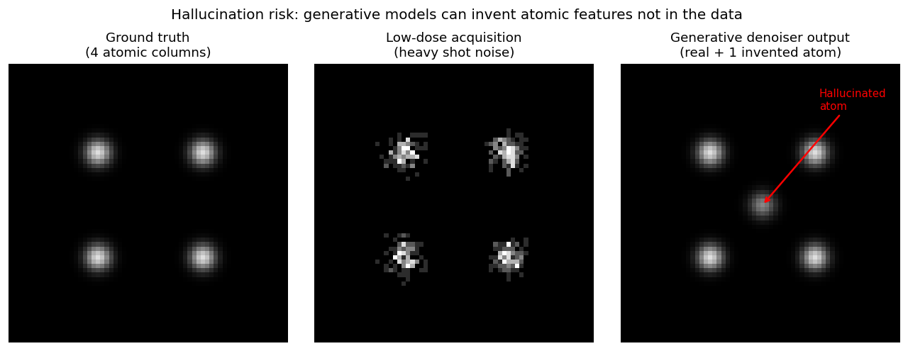
Hallucination risk: a low-dose HAADF image (centre) has four real atomic columns with heavy shot noise. A generative denoiser (right) recovers the four true columns but also invents a fifth (red arrow) in the centre — a feature with no ground-truth basis (left). This is the hallucination failure mode: the model’s learned prior places a plausible atom at the centre because it “looks like” an atom should be there, not because the data supports it.

• Walk through the three panels carefully. The ground truth (left) has four columns at the corners — nothing in the centre. The raw measurement (centre) is dominated by noise — no clear column positions visible. The GAN/diffusion output (right) correctly recovers the four true columns but also places a fifth at the centre.
• Why did the denoiser invent the fifth atom? The prior probability of a symmetric 5-atom cluster (corners + centre) was higher in the training data than a 4-atom cluster (corners only). The noisy centre region provided slight support for something there. The network “filled in” the most probable completion — which happened to be wrong.
• The inability to distinguish this from a correct reconstruction by visual inspection alone is the core problem. Both the correct reconstruction (4 atoms) and the hallucinated one (5 atoms) look “physically reasonable” and “clean.” Only comparison to the ground truth (or very high-dose re-measurement) reveals the error.
• Prevention strategies: (1) quantify reconstruction uncertainty (use an ensemble of denoised outputs — consistent features are likely real); (2) validate key features at higher dose; (3) use physics constraints that make a 5th atom penalised if no electron scattering supports it.

Distribution shift: when the training data does not match the specimen

• Distribution shift: the generative model was trained on specimens from distribution \(p_{\text{train}}\). The test specimen comes from \(p_{\text{test}} \neq p_{\text{train}}\).
• EM examples:
  • GAN trained on perfect SrTiO\(_3\) applied to a SrTiO\(_3\) specimen with a grain boundary → grain boundary erased.
  • VAE trained on Au nanoparticles applied to a Pt-Au alloy → Pt columns reconstructed as Au.
  • Diffusion model trained on room-temperature images applied to a cryogenic sample → ice contamination reconstructed as carbon contamination.
• How to detect: compare the residual (measurement − forward model(reconstruction)) to the expected Poisson noise. If the residual has systematic structure, the reconstruction is wrong.
• Mitigation: train on a diverse dataset, including out-of-distribution examples; report uncertainty estimates; always show the residual map alongside the reconstruction.

• Distribution shift is the most common failure mode in practice. The training data is almost never a perfect match for the test specimen — different microscope, different sample preparation, different dose, different crystal orientation.
• The residual check is the most reliable quality metric: if \(H(\hat{x}) = y\) within noise statistics, the reconstruction is self-consistent. If the residual has structure (peaks where atoms “should be” but weren’t reconstructed, or smooth regions where the reconstruction placed atoms), there is a problem.
• Uncertainty quantification is the research frontier: instead of producing one reconstruction, produce an ensemble of 10 reconstructions with different noise seeds, or use MC-Dropout in the denoiser. Pixels/regions where the ensemble disagrees strongly are uncertain — do not interpret them as real structure.
• The “patient safety” analogy: a doctor who over-diagnoses (hallucinates tumors) and a doctor who under-diagnoses (misses tumors) are both dangerous. A reconstruction that confidently shows wrong structure is worse than a noisy reconstruction that honestly reflects uncertainty.

When NOT to trust a generative reconstruction

• Red flags — treat the output with extreme caution:
  1. Dose is very low (\(< 10^2\) e⁻/Ų) and the reconstruction looks suspiciously perfect (no noise).
  2. You see a feature (defect, interface, precipitate) not present in the training data.
  3. The residual map shows systematic patterns — the reconstruction does not fit the measurement statistics.
  4. The reconstructed feature would be the most important result in your paper — validate it independently.
• Green flags — higher confidence:
  1. The reconstruction is consistent across multiple noise seeds (ensemble agreement).
  2. The residual is consistent with the expected noise model (Poisson at low dose).
  3. The key features were also visible in a high-dose reference image.
  4. A physics-informed constraint (e.g., known crystal symmetry) was enforced.

• The “most important result in your paper” red flag is intentionally provocative. In scientific reporting, the tendency is to emphasise the most striking finding. But generative models are most likely to hallucinate precisely in the most striking regions — where the prior has the most influence relative to the data.
• The Poisson residual check is quantitative: after reconstruction, compute \(r_i = (y_i - H(\hat{x})_i) / \sqrt{H(\hat{x})_i}\) (normalised residual for Poisson noise). Each \(r_i\) should be approximately \(\mathcal{N}(0,1)\) if the reconstruction is correct. The mean and variance of \(r\) should be 0 and 1 respectively. A mean \(\neq\) 0 signals systematic bias; variance > 1 signals over-smooth reconstruction.
• The ensemble agreement check is practically useful: run the generative reconstruction 5–10 times with different random seeds (for diffusion) or dropout patterns (for MC-Dropout). Average the reconstructions. The per-pixel variance measures uncertainty. High-variance regions are not reliable.

The reliability spectrum: classical vs learned vs physics-informed

• Classical regularisation (Tikhonov/TV): fully interpretable, predictable failure modes (smoothing bias), no training data needed. Conservative but reliable. Best for: sparse data, well-known prior (smooth or piecewise-constant), need for certified uncertainty.
• Physics-informed learning: exploits physical laws, can extrapolate beyond training data if physics is correct. Dangerous when physics model is wrong. Best for: known PDE/ODE, data-limited regime, physical consistency required.
• Generative model prior (VAE/GAN/diffusion): highest quality, can capture complex real-world structure. Most dangerous — hallucination and distribution shift are hard to detect. Best for: large training set, similar test specimens, quality over certified reliability.
• Bottom line: always report which method was used, at what dose, and with what validation. “AI-enhanced EM” is only credible when the uncertainty and validation are explicit.

• The “credibility” framing is important for scientific communication. There is growing concern in the EM community (and beyond) about AI-enhanced results that look compelling but cannot be verified. The responsibility is on the author to provide the validation evidence.
• The “certified uncertainty” distinction: classical methods have mathematical guarantees — Tikhonov gives a bounded RMSE as a function of \(\lambda\) and the condition number. Generative methods have no such guarantees — the hallucination rate is an empirical property of the trained model and the test distribution.
• For the exam: the key comparison table question is “when do you choose each method?” Use the slide bullet points as the answer template.

Uncertainty quantification: making generative models trustworthy

• The core problem: a single generative reconstruction gives one answer with no error bar. The answer might be right or it might be a hallucination — the output looks identical in both cases.
• Ensemble approach: run the reconstruction multiple times with different random seeds (diffusion) or Monte-Carlo dropout (GAN/VAE). High-confidence features appear consistently; hallucinated features are inconsistent across runs. Report per-pixel variance alongside the mean.
• Residual-based confidence: compute \(r = (y - H(\hat{x})) / \sqrt{H(\hat{x})}\). If \(r \sim \mathcal{N}(0,1)\) everywhere (Poisson noise), the reconstruction is self-consistent. Systematic structure in \(r\) signals that the model has over-fitted the prior.
• Physics-constrained uncertainty: combine a generative prior with a physics residual constraint. The physics restricts the hallucination space — a hallucinated atom that violates the known scattering model is penalised. This is the current frontier in ptychography + learned-prior methods. Pelz, Philipp M. et al., (2021), doi:10.1038/s41467-021-22204-1

• The ensemble approach is the most practically accessible. It requires no additional training — just running inference multiple times. For diffusion models, different noise seeds produce different “denoising paths” that all pass through the same measurement-consistent constraint but diverge in uncertain regions.
• The per-pixel variance map from an ensemble is a pseudo-uncertainty estimate — it quantifies “how much do different runs disagree” rather than the full posterior variance. It is a proxy, not a mathematically certified uncertainty, but it is practical and widely used.
• The physics-constrained uncertainty is conceptually the cleanest: if you add \(\lambda\|\mathcal{F}[f_\theta]\|^2\) to the generative prior loss, hallucinations that violate known physics are suppressed. The remaining uncertainty is about physical configurations that are both consistent with the data AND satisfy the physics model — a well-defined class.
• For the exam: the key concept is “ensemble disagreement = uncertainty”. Students should be able to describe the ensemble approach and explain why consistent features are more trustworthy than inconsistent ones.

Choosing a reconstruction method

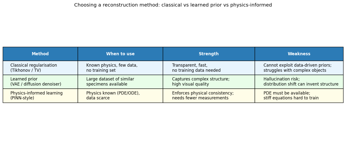
Decision table: classical regularisation (Tikhonov/TV) for well-understood physics and limited data; learned prior (VAE/GAN/diffusion) when a large dataset of similar specimens is available; physics-informed learning when the governing equations are known and data is scarce. The three approaches are complementary; combining them (e.g., physics-informed GAN) is an active research direction.

• Walk through each row. Row 1 (classical): this is the default for new/unusual specimens where no training data exists. Tikhonov is the “safe” baseline. TV is better for piecewise-constant specimens (atomic columns in vacuum). Both can be run in minutes on a laptop.
• Row 2 (learned prior): this is the high-performance option when you have a curated training set from the same instrument, material class, and dose range. The quality is much better but the failure modes are more subtle.
• Row 3 (physics-informed): this is the right choice when you know the governing equation (Schrödinger, Poisson, diffraction geometry) and have limited measurements. It is the current state of the art for ptychographic tomography where the multislice model is used as the forward operator.
• The combination row: physics-informed GANs are an active research direction — the GAN generator must produce structures that satisfy the physics model (hard constraint) and look like real data (adversarial loss). Early results are promising but the training is difficult (two objectives that can conflict).

A practical decision guide for EM reconstruction

• Start with: what is your dose? If dose is high (> 10⁴ e⁻/Ų), most methods work — prefer the fastest.
• If dose is low: generative methods are tempting but most dangerous. Use physics-informed or classical as a benchmark; add generative only if it passes the residual check.
• If you have training data: compute the distribution shift — do training images look like test images (similar defect density, orientation, element, dose)? If yes, generative is safe. If uncertain, use classical as a baseline and compare.
• If speed matters: classical (seconds/minutes) > PINN (minutes) > GAN/diffusion (minutes to hours).
• Always report: method name, training data description, dose, residual map, key assertion validated at higher dose.

• The “always report” list is the scientific standard that the community is converging on. Several leading EM journals (Ultramicroscopy, Microscopy and Microanalysis) now require explicit uncertainty quantification for AI-enhanced reconstructions.
• The “higher dose validation” is the gold standard: if you claim a defect from a generative reconstruction at 100 e⁻/Ų, go back and image the same area at 10⁴ e⁻/Ų (if the material can survive it). If the defect is still there, you have validation. If it disappears, it was a hallucination.
• The speed hierarchy is important for experimental workflows. Ptychographic reconstruction of a 64×64 scan with ePIE takes ~10 s on a modern CPU. A GAN super-resolution inference takes ~1 s (once trained). A diffusion reconstruction takes ~10 min per image. Plan acquisition strategies accordingly.

Week 12 synthesis

• Ptychography: phase retrieval from overlapping probe measurements is the premier example of a physics-driven solution to the inverse problem — the over-determined forward model uniquely constrains the phase. No learning required.
• Physics-informed learning: add the physics residual \(\lambda\|\mathcal{F}[f_\theta]\|^2\) to the reconstruction loss. Exploits known equations, works with limited data, fails when the physics model is wrong.
• Generative priors (VAE/GAN/diffusion): the most powerful and most dangerous tools. Learned from data, can produce stunning reconstructions, but will hallucinate structure when data is insufficient or out-of-distribution.
• The meta-lesson: more powerful = more assumptions. Every algorithm that improves on the raw noisy measurement is making assumptions about what the “true” object looks like. The assumption must be stated, tested, and reported.
• Self-study: run week12_ptychography_forward.ipynb — step sizes 4/6/8 px, observe amplitude-consistency error 0.0991→0.0021 / 0.1048→0.0067 / 0.1008→0.0091; assert more overlap → lower error — all genuine.

• The meta-lesson is the take-away sentence for Week 12. Write it on the board: “More powerful = more assumptions.” Students should be able to apply this heuristic to any reconstruction algorithm they encounter in the literature.
• The progression of the course: Week 1–4 (data and learning basics) → Week 5–8 (supervised and unsupervised ML) → Week 9–10 (probabilistic + active acquisition) → Week 11 (classical inverse problems) → Week 12 (modern/advanced inverse problems) → Week 13 (explainability and trust). The narrative arc: we built more and more powerful tools; Week 13 asks “when do we trust them?”
• The connection to Week 13 is intentional: explainability and trust are the answers to the “meta-lesson.” Attribution methods (SHAP, GradCAM) tell you WHY the network made a specific choice. Calibration tells you HOW reliable the uncertainty estimates are. Both are forms of “stating and testing the assumptions.”

Forward link: Week 13 — Explainability, trust & synthesis

• Week 13 will address: how do we know why an ML model made a particular reconstruction choice? When can we trust a model’s output for scientific conclusions? How does Week 13 synthesise the full 13-week course?
• The questions raised this week:
  • A generative model hallucinates — how do we know which features to trust?
  • A physics-informed reconstruction has residual error — is it due to a wrong physics model or measurement noise?
  • A ptychographic reconstruction converges — but to which of the many local minima?
• Week 13 tools: attribution methods (GradCAM, SHAP) for identifying which pixels drove a reconstruction; calibration methods (conformal prediction, Platt scaling); and a synthesis of the full DSEM framework.
• Exam prep: _shared/exam_mustknow.md Week 12 section is now populated — review before Week 13.

• The three “questions raised this week” are the specific threads Week 13 picks up. For ptychography: the ePIE algorithm can have multiple local minima (especially with insufficient overlap or poor initialisation). Explainability can help identify which parts of the measurement most constrained the reconstruction. For generative models: attribution maps can show which pixels of the noisy input “supported” each feature of the reconstruction — features with no supporting evidence in the input are hallucinations.
• The course synthesis in Week 13: the 13-week arc from “what is an array” to “when do I trust my AI reconstruction” is a complete introduction to data science for EM. Week 13 closes the loop by asking students to apply every concept to a single integrated pipeline — from raw 4D-STEM data to a trusted, explainable, uncertainty-quantified structural conclusion.
• Practical exam prep reminder: the exam_mustknow.md file now has Week 12 entries. Students should be able to: (1) describe the ptychographic forward model formula; (2) explain ePIE in 3 steps; (3) name the three generative model families and one EM application of each; (4) describe two hallucination risk indicators; (5) compare the three reconstruction approaches in a table.

Continue

• ← Back: Week 11 — Imaging inverse problems I
• → Next: Week 13 — Explainability, trust & synthesis
• All courses

References

Hard-x-ray lensless imaging of extended objects, Physical Review Letters, John M. Rodenburg, A. C. Hurst, A. G. Cullis, B. R. Dobson, F. Pfeiffer, O. Bunk, C. David, K. Jefimovs, & I. Johnson https://doi.org/10.1103/PhysRevLett.98.034801.

An improved ptychographical phase retrieval algorithm for diffractive imaging, Ultramicroscopy, Andrew M. Maiden & John M. Rodenburg https://doi.org/10.1016/j.ultramic.2009.05.012.

Electron ptychography achieves atomic-resolution limits set by lattice vibrations, Science, Zhen Chen, Michal Odstrcil, Yi Jiang, Yimo Han, Ming-Hui Chiu, Lain-Jong Li, & David A. Muller https://doi.org/10.1126/science.abg2533.

A plug-and-play image reconstruction framework, IEEE Signal Processing Magazine, Ulugbek S. Kamilov, Charles A. Bouman, Gregery T. Buzzard, & Brendt Wohlberg https://doi.org/10.1109/MSP.2022.3199595.

Physics-informed neural networks: A deep learning framework for solving forward and inverse problems involving nonlinear partial differential equations, Journal of Computational Physics, Maziar Raissi, Paris Perdikaris, & George E. Karniadakis https://doi.org/10.1016/j.jcp.2018.10.045.

Auto-encoding variational Bayes, arXiv preprint arXiv:1312.6114, Diederik P. Kingma & Max Welling.

Generative adversarial nets, Advances in neural information processing systems, Ian Goodfellow, Jean Pouget-Abadie, Mehdi Mirza, Bing Xu, David Warde-Farley, Sherjil Ozair, Aaron Courville, & Yoshua Bengio.

Denoising diffusion probabilistic models, Advances in neural information processing systems, Jonathan Ho, Ajay Jain, & Pieter Abbeel.

Solving complex nanostructures with ptychographic atomic electron tomography, Nature Communications, Philipp M. Pelz, Wei Xiang Qiu, Robert Bücker, Günther Kassier, & R. J. Dwayne Miller https://doi.org/10.1038/s41467-021-22204-1.