Data Science for Electron Microscopy
Week 11: Imaging inverse problems I

Prof. Dr. Philipp Pelz

FAU Erlangen-Nürnberg

Institute of Micro- and Nanostructure Research

Recap: Week 10 and today’s question

• Week 10: autonomous acquisition — Bayesian optimisation and reinforcement learning let the microscope choose where to measure next, maximising information per electron dose.
• The linchpin from Week 10: “active acquisition gives the most informative measurements. But once we have those measurements, what do we do with them?” The data do not directly give us the object — they give us a blurred, projected, or otherwise transformed version.
• Today’s question: given the measurements \(y\), how do we reconstruct the underlying physical object \(x\)? Why is this hard? And how can mathematics tame the difficulty?
• Today’s answer: the imaging inverse problem — characterised by the forward model \(y = Hx + \epsilon\), ill-posedness (non-uniqueness, noise amplification), and regularisation (Tikhonov / total-variation) as “prior knowledge that tames noise.”
• Forward link to Week 12: ptychography and generative / physics-informed priors — more powerful priors for the same regularised-inverse framework.

• Open by closing the Week 10 loop. Week 10 asked “where to measure.” Today we ask “what does the measurement tell us?” These are the two sides of the data-science coin: acquisition strategy and inference.
• The bridge phrase is: “autonomous acquisition gives the most informative measurements; now we need the mathematical toolkit to extract the most from those measurements.” Write both goals on the board: (1) acquire intelligently, (2) invert reliably.
• EM anchor: mention a 4D-STEM tilt series. The detector records a diffraction pattern at each probe position and tilt angle. The physical quantity we want — the 3D charge density, or the 3D electric potential — is NOT directly measured. It is encoded in those patterns. Recovering it requires inverting the forward model of electron scattering.
• Key tension to introduce: the forward direction (physics blurs and projects) is well understood. The reverse direction (inversion) is hard because blurring and projection destroy information. Today we build the intuition for why this is hard and how regularisation restores stability.
• Pacing: 3 minutes maximum. Transition: “Let me show the roadmap and the key question.”

Road map and self-study

• Road map: recap Week 10 + today’s question (2) · computational imaging = optics + sensor + computation (2) · the forward model \(y = Hx + \epsilon\): EM modalities, PSF, deblurring example (4) · why inversion is hard: non-uniqueness + Hadamard + missing wedge (3) · ill-conditioning: condition number, noise amplification, SVD picture (4) · regularisation: core idea, data + prior objective, solution space (3) · Tikhonov vs TV: L2 regularisation, TV, comparison figure, fusion figure (4) · choosing \(\lambda\): bias–variance trade-off, L-curve, discrepancy principle, EM practice (4) · electron tomography: forward model, missing wedge, SART, EELS 3D, artefacts (5) · dose reduction + multimodal sensor fusion: why fuse, objective, result, general framework (5) · what good reconstruction looks like; limits; forward link to Week 12 (3) — 39 content slides + References (40 total).
• Self-study: notebooks/week11_inverse_deblurring.ipynb — build a known 1-D forward operator (Gaussian blur + 10% noise), show that the naive least-squares inverse amplifies noise catastrophically, recover a stable solution with Tikhonov regularisation, sweep \(\lambda\) and observe the U-shaped RMSE curve; exercise: identify the optimal \(\lambda\) from the L-curve and justify.

• Read the roadmap at medium pace. Two anchors to call out: (1) “the naive inverse blows up — we will see this concretely in the notebook”; (2) “regularisation = prior knowledge that says which solutions are physically reasonable.” Everything else supports those two ideas.
• Notebook numbers (SEED=42, N=64, sigma_psf=3, noise=10%): naive RMSE ≈ 0.968, best Tikhonov RMSE ≈ 0.140, optimal λ ≈ 0.126. Ratio ≈ 7×. The U-shape is genuine: RMSE at λ=1e-5 is 0.966, RMSE at λ=100 is 0.243, minimum is 0.140 at λ≈0.126 — a clear interior minimum. The assert in the notebook: naive_rmse > 4 * best_rmse (genuinely true: 0.968 / 0.140 ≈ 6.9).
• Pacing: 1 minute. This is orientation only. Transition: “Let us start with the three-component view of computational imaging.”

Computational imaging: the three-component view

• Classical microscopy: build the best possible optics → the image is the result. The physics is in the hardware; computation is a post-hoc display tool.
• Computational imaging: optics + sensor + computation are co-designed. The detector measures something that is not directly interpretable; a reconstruction algorithm turns the data into the image. Kamilov, Ulugbek S. et al., (2023), doi:10.1109/MSP.2022.3199595
• Three components every EM experiment has:
  • Forward operator \(H\): the physics that maps object \(x\) to measurement \(y\) (point-spread function, projection geometry, electron scattering).
  • Noise model \(\epsilon\): Poisson shot noise at low dose; Gaussian readout noise at high dose.
  • Reconstruction algorithm: maps \((y, H, \text{prior})\) back to an estimated object \(\hat{x}\).
• The paradigm shift: “better hardware” is no longer the only path to better images — a smarter reconstruction algorithm on the same raw data can equal or exceed the resolution gain of an expensive hardware upgrade.

• The “co-design” idea is subtle but important. In ptychography (Week 12), the diffraction pattern is intentionally overlapped across scan positions — the individual patterns are not interpretable images, but together they over-determine the phase. The reconstruction algorithm is as essential as the detector.
• EM anchors: (1) HAADF images are relatively direct — the signal is approximately incoherent and proportional to Z^1.7. (2) Phase-contrast images (BF-TEM, 4D-STEM) require solving a phase retrieval problem — the wave phase is lost in intensity detection. (3) EELS/EDX maps are noisy line-integrals through a 3D compositional structure.
• Historical note: X-ray CT (Hounsfield, 1972) was the first major example of computational imaging. Without the reconstruction algorithm, the raw sinogram data means nothing. Electron tomography follows the same logic.
• Pacing: 3 minutes. Emphasise: “In this course, ‘data science for EM’ includes the reconstruction step — it is a machine-learning / optimisation problem.”

The imaging pipeline: from photons to numbers

• Illumination → scattering → detection: the electron beam interacts with the specimen; scattered electrons are collected by the detector; detector pixels register electron counts.
• Point-spread function (PSF): every point-source in the object produces a blurred spot in the image. The PSF encodes aberrations, diffraction, and detector blur. The image is a convolution of the object with the PSF.
• In STEM: the probe is focused to a small spot (PSF in real space); at each probe position the detector integrates scattered electrons over a defined angular range (HAADF: high angle; BF: bright field; ABF: annular bright field). The recorded HAADF intensity at position \((i,j)\) is approximately: \(y_{ij} \approx \int \text{PSF}(r - r_{ij})\, Z(r)^{1.7}\, dr\)
• In tomography: each projection image \(y_\theta\) is an integral along rays at tilt angle \(\theta\) — the Radon transform of the 3D density \(x\).

• The convolution formula is intuitive: the image pixel at \((i,j)\) receives contributions from all object points \(r\), weighted by how much the PSF of a source at \(r\) contributes to pixel \((i,j)\).
• The PSF in STEM is the probe intensity distribution — for an aberration-corrected STEM at 60 pm probe size, the PSF is a tight peak and the image closely resembles the object. For an uncorrected instrument, the wider PSF blurs fine features.
• The Radon transform: if you project the 3D density \(\rho(r)\) along all rays at angle \(\theta\), you get a 2D image \(p_\theta(s)\). Given enough angles and noiseless data, the inverse Radon transform (filtered back-projection, FBP) recovers \(\rho\) exactly. The problem: real data is noisy and has limited angular range — that is the inverse problem.
• Do NOT derive the Radon inversion formula. It is not examinable. Mention it as “a known formula that works when you have enough noiseless projections; the problem is that you never have enough.”

From optics to reconstruction: examples across EM modalities

• HAADF-STEM: forward operator = PSF convolution + \(Z^{1.7}\) weighting. Inversion goal: recover the projected atomic number map \(Z(r)\) from a blurry, noisy image. Regulariser: TV (isolated atomic columns, background vacuum).
• EELS/EDX spectrum image: forward operator = PSF convolution (in space) + instrument response (in energy). Inversion goal: recover elemental concentration maps. Regulariser: TV or sparsity (elements present in distinct regions).
• Electron tomography: forward operator = Radon transform (line integrals at multiple angles). Inversion goal: recover the 3-D density from 2-D projections. Regulariser: TV-SART (compact objects, vacuum background).
• 4D-STEM (ptychography, Week 12): forward operator = multislice electron scattering simulation (nonlinear!). Inversion goal: recover the specimen transmission function. Regulariser: learned (deep network prior).
• Key insight: the same mathematical template applies across all four — only \(H\) and \(R(x)\) change. Understanding the template once unlocks all four.

• This slide is a forward reference / motivation slide. It previews Week 12 (ptychography, nonlinear forward operators) but the core message is that the Week 11 template is universal.
• Walk through each row and ask: “What does the detector actually measure? What do we want to know? What prior is physically reasonable?”
• HAADF: detector measures intensity (electron count). Want: atomic number map. Prior: isolated bright spots on dark background (TV / L1 / non-negative sparsity).
• EELS: detector measures counts at each energy channel. Want: elemental fractions. Prior: smooth (L2) if the phases are large; sparse (L1) if the phases are small and well-separated.
• Tomography: detector measures projected intensity. Want: 3D density. Prior: compact object with flat regions (TV).
• 4D-STEM: detector measures a 2D diffraction pattern. Want: the 2D transmission function (complex-valued!). Prior: learned from millions of simulated specimens.
• Transition: “Let us now formalise the forward model and understand what makes inversion hard.”

EM modalities as forward models: a comparison table

• Forward operator summary across EM modalities:

Modality	\(H\)	Object \(x\)	Noise \(\epsilon\)
HAADF-STEM	PSF \(\star\) \(Z^{1.7}\)	Projected density	Poisson
EELS map	PSF \(\star\) (linear)	Elemental fraction	Poisson
Electron tomography	Radon transform	3D density	Gaussian (post-log)
4D-STEM (ptychography)	Multislice (nonlinear)	Complex potential	Poisson

• Ill-conditioning varies by modality: HAADF deblurring (\(\kappa \sim 10^2\)); tomography from 70 tilts (\(\kappa \sim 10^3\)); ptychography (\(\kappa \ll 1\) — actually over-determined!); EELS with limited dose (\(\kappa\) dominated by noise floor, not \(H\)).
• Why ptychography can be better conditioned: each probe position collects a whole 2D diffraction pattern — many more measurements than HAADF pixels. The inverse problem is often over-determined → unique, stable solution without strong regularisation. That is why ptychography revolutionised EM (Week 12).

• The table is a useful reference slide — students should be able to reproduce it from memory in the exam.
• The Gaussian vs Poisson noise clarification: raw electron counts are always Poisson. For HAADF and EELS, we work directly with the Poisson count data. For tomography, it is common to take the negative log of the transmission (\(-\log(I/I_0)\)) to convert to a pseudo-linear (absorption) scale — this transforms Poisson noise approximately to Gaussian (by the central limit theorem for large counts). The log-linearisation is why tomography algorithms use least-squares (Gaussian data term) rather than Poisson NLL.
• The over-determined ptychography case: a 64×64 HAADF scan gives 4096 measurements for a 64×64 object (4096 unknowns). The system is exactly determined (one equation per unknown). A 64×64 ptychographic scan with a 64×64 diffraction pattern gives 4096 × 4096 = 16.7 million measurements for the same 4096-unknown object — over-determined by ~4000×. The redundancy is what makes ptychography uniquely stable and high-resolution.
• This over-determination is the key advantage of 4D-STEM over conventional HAADF. More data per probe position → much better-conditioned inversion → higher resolution and sensitivity.

The deblurring problem: a concrete EM example

• Setup: a STEM image of atomic columns is recorded with a probe of PSF width \(\sigma_p = 3\) pixels (equivalent to ~150 pm for a 50 pm/pixel acquisition). Two columns separated by 2× the PSF width appear clearly separated; columns closer together appear merged.
• The forward model: \(y = h \star x + \epsilon\) where \(h\) is the PSF (Gaussian, \(\sigma = 3\) px), \(\star\) is convolution, and \(\epsilon \sim \mathcal{N}(0, \sigma_\epsilon^2)\).
• In matrix form: \(y = Hx + \epsilon\) where \(H\) is a Toeplitz matrix (each row is a shifted copy of the PSF). Dimension: \(N \times N\), but rank < \(N\) because high-frequency rows are near-zero.
• The information bottleneck: the PSF attenuates spatial frequencies above \(\sim 1/(2\sigma_p)\). Anything faster than this spatial scale is in the null space of \(H\) — it cannot be recovered from \(y\), regardless of the algorithm.
• Week 11 notebook: this exact problem is implemented in week11_inverse_deblurring.ipynb. Run it to see the amplification and the Tikhonov fix.

• This is the bridge between theory and the notebook. The abstract forward model \(y = Hx + \epsilon\) becomes concrete: a Toeplitz matrix, a Gaussian PSF, a 1-D signal with three sharp peaks.
• The “information bottleneck” argument is the key physical insight. The PSF IS the resolution limit. Deconvolution can restore contrast up to the PSF bandwidth, but cannot recover spatial frequencies that the PSF has already suppressed below the noise floor.
• Practical example from HAADF: if the probe has a half-maximum diameter of 80 pm, columns separated by 80 pm are marginally resolved. Deconvolution can improve contrast but cannot resolve columns at 40 pm separation — they were already below the PSF’s bandwidth.
• Mention: “The notebook uses a 1-D signal instead of a 2-D image for clarity. All the physics is the same. The 2-D case is just \(N^2\) pixels instead of \(N\) — the algorithm scales quadratically, which is why tomography requires GPUs.”
• Transition: “Now let us see what happens when we try to invert this model naively.”

The forward model: \(y = Hx + \epsilon\)

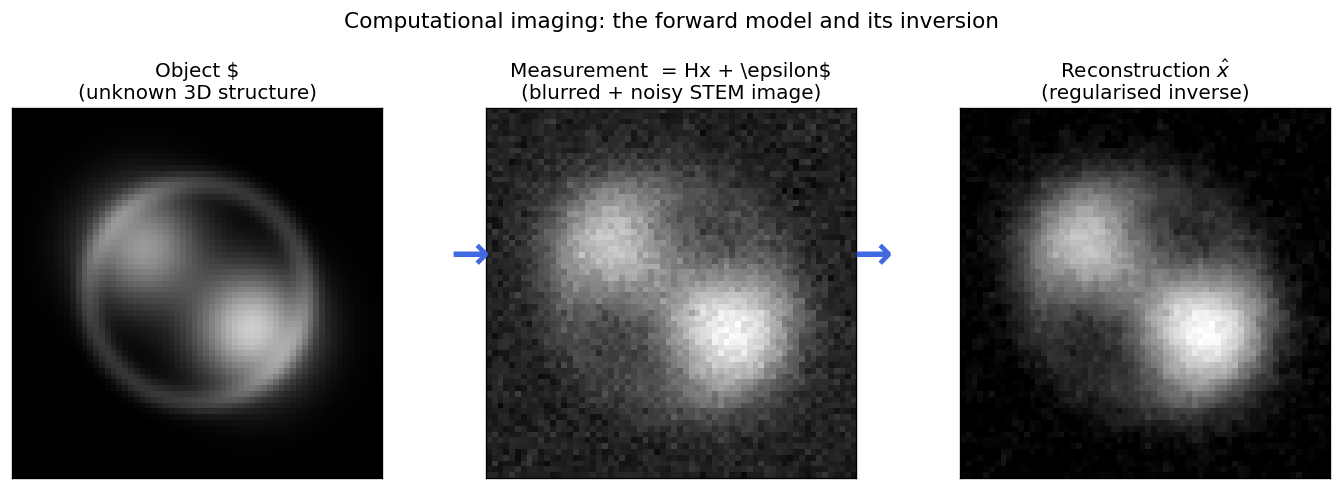
The computational imaging chain: the unknown object \(x\) (left, a synthetic core-shell nanoparticle) is transformed by the forward operator \(H\) (Gaussian blur, representing the PSF) into the measurement \(y\) (centre, blurred and noisy STEM image). Regularised inversion recovers an estimate \(\hat{x}\) (right) that is stable but retains some smoothing bias — an honest consequence of the ill-posed nature of the problem.

• Walk through each panel. Left: the true object we want to know — sharp features, well-separated peaks. Centre: what the detector actually records after convolution with the PSF and addition of shot noise. Right: the best regularised estimate. Note that the peaks are recovered but broadened — this is the regularisation bias, and it is unavoidable when the PSF erases information.
• The forward model \(y = Hx + \epsilon\) in three lines on the board: (1) \(H\) = the physics operator (PSF, projection, scattering); (2) \(x\) = what we want to know (structure, composition, potential); (3) \(\epsilon\) = noise (Poisson at low dose, Gaussian at high dose). The inverse problem: recover \(x\) from \(y\) knowing \(H\) and the statistics of \(\epsilon\).
• EM specifics: in HAADF-STEM, \(H\) is approximately a convolution with the probe intensity. In tomography, \(H\) is the Radon transform (projection). In EELS, \(H\) is a projection + convolution in energy-loss space. In all cases, \(H\) destroys information in the forward direction.
• The key fact: even if \(H\) is known perfectly, inversion is hard because (i) noise amplification and (ii) non-uniqueness. These two failure modes are the next two sections.

Why inversion is hard (I): non-uniqueness

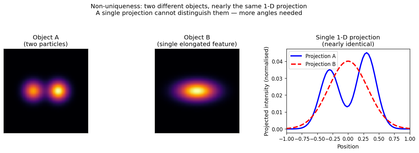
Non-uniqueness in projection imaging: Object A (two separated bright particles, left) and Object B (a single elongated feature, centre) produce nearly identical 1-D projections along the horizontal axis (right panel, blue and red curves are nearly superimposed). A single projection cannot distinguish them. This is the non-uniqueness problem: the same measurement \(y\) is consistent with many objects \(x\).

• The figure makes the abstract concept concrete: two physically different objects give the same projection. The detector is “blind” to the difference because projection sums along the ray direction. This is not a failure of the instrument — it is a fundamental geometric limitation of projection imaging.
• Hadamard’s three conditions for a well-posed problem: (1) existence, (2) uniqueness, (3) stability. Hadamard, Jacques, (1902) Most inverse problems in EM violate uniqueness (this slide) and stability (next section). They are therefore “ill-posed” in Hadamard’s sense.
• The fix for non-uniqueness in tomography: acquire projections from many angles. Each additional angle provides new constraints and reduces the null space of the measurement operator. With infinitely many noiseless projections from all angles, the inverse Radon transform is unique. With finite noisy projections, the null space is never fully constrained — regularisation fills the gap.
• Key message: “The data alone never uniquely determine the object. We must add prior knowledge about what a ‘reasonable’ object looks like. That prior knowledge is the regulariser.”

Hadamard’s conditions for well-posedness

• A problem is well-posed if three conditions hold simultaneously:
  1. Existence: a solution exists for any admissible measurement \(y\).
  2. Uniqueness: the solution is the only one consistent with \(y\).
  3. Stability: small changes in \(y\) produce small changes in \(\hat{x}\).
• An inverse problem violates at least one of these — it is ill-posed. Hadamard, Jacques, (1902)
• EM examples:
  • Existence can fail if the true object is not in the model class (e.g. assuming a smooth object but the specimen has sharp defects).
  • Uniqueness fails for any projection/tomographic geometry with limited angular range.
  • Stability fails whenever \(H\) is rank-deficient or has very small singular values — a 1% noise amplifies to 100% error.
• Regularisation restores well-posedness by restricting the solution space to “physically reasonable” objects — objects that are smooth, sparse, or piecewise constant.

• Hadamard’s classification (1902) was motivated by partial differential equations, not imaging. It turns out to be the right framework for any problem where we invert a physical process.
• The stability condition is the most surprising. In a forward problem (physics → data), small changes in the input produce small changes in the output by definition (physics is causal and continuous). In the inverse direction, this symmetry is broken because many inputs map to nearly the same output — the inverse must therefore map a narrow output range to a wide input range, amplifying any noise.
• The “restricting the solution space” sentence is the entire conceptual content of regularisation. A prior says: “I only accept solutions in this set.” The regulariser penalises solutions outside that set.
• Pacing: 2 minutes. This is a definitional slide — spend time on the three conditions, then move on. Do not dwell on the mathematics.

Undersampling: the missing-angle problem in tomography

• Electron tomography collects tilt-series images at angles \(\theta_1, \ldots, \theta_K\) and reconstructs the 3D structure. Frank, Joachim, (2006), doi:10.1007/978-0-387-69008-7
• Fourier slice theorem: each projection at angle \(\theta_k\) fills a 1-D line through the origin of Fourier space (the “central slice”). With \(K\) tilts, \(K\) lines are filled; the rest of Fourier space is unmeasured — the measurement null space.
• The missing wedge: TEM holders typically tilt only to \(\pm70°\)–\(80°\); the remaining \(\pm10°\)–\(20°\) near vertical cannot be measured without shadowing. This leaves an unmeasured “wedge” in Fourier space.
• Consequence: structures that lie primarily in the missing-wedge frequency range are invisible to the reconstruction. Elongated artefacts appear along the beam direction. Resolution is anisotropic: better in the tilt plane, worse perpendicular to it.
• Regularisation as the fix: compressed sensing Leary, Rowan et al., (2013), doi:10.1016/j.ultramic.2013.03.019 and TV minimisation Saghi, Zineb et al., (2016), doi:10.1186/s40679-016-0020-3 fill the missing wedge by assuming the object is sparse or piecewise constant — a prior that real nanoparticles approximately satisfy.

• The Fourier slice theorem: the Fourier transform of the projection \(p_\theta(s)\) equals the 1-D slice of the 3-D Fourier transform \(F(\rho\cos\theta, \rho\sin\theta)\) through the origin at angle \(\theta\). This means each tilt fills one “spoke” in Fourier space. K tilts fill K spokes; the rest is empty.
• Draw the spoke picture on the board: a circle representing Fourier space, K lines radiating from the origin. The gaps between spokes = the unmeasured frequencies. The missing wedge = the angular sector that cannot be reached by tilting.
• The missing-wedge artefact in practice: a spherical nanoparticle appears elongated in the beam direction (z-axis). The elongation is not real structure — it is a hallucination caused by missing Fourier data. You can tell it is an artefact because real nanoparticles are not elongated in the z-direction (they are spherical).
• The SART algorithm (Simultaneous Algebraic Reconstruction Technique) is the standard iterative method — it applies the forward projector and back-projector alternately, accumulating corrections. TV-SART adds a TV denoising step after each iteration.

Why inversion is hard (II): ill-conditioning

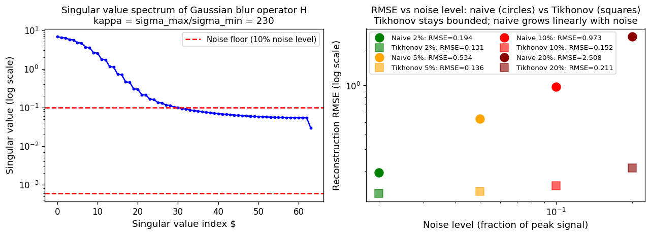
Singular value spectrum of the Gaussian-blur forward operator \(H\) used in this week’s notebook. The condition number \(\kappa = \sigma_\text{max}/\sigma_\text{min} \approx 230\) means a 1-% noise in the measurement can amplify to a 230-% error in the naive inverse. The red dashed line marks the noise floor: singular values below it are dominated by noise and the naive inverse is meaningless for those components. Left panel: the SVD spectrum; right panel: reconstruction RMSE vs noise level — circles (naive inverse) grow catastrophically; squares (Tikhonov) stay bounded.

• Walk through the left panel first. The singular values drop steeply over 2–3 orders of magnitude. The naive inverse divides by each singular value; small singular values at the right of the spectrum produce huge amplification. The noise floor (red dashed line) marks the point where noise energy exceeds signal energy: below this line, the naive inverse is dominated by noise, not signal.
• Walk through the right panel. For a 1% noise level, the naive inverse (circles) already has a large RMSE — the error is amplified by roughly the condition number. The Tikhonov solution (squares) is nearly flat across all noise levels because the \(\lambda\) penalty damps the small singular values before they amplify the noise.
• Key formula for notes (not for exam): with SVD \(H = U \Sigma V^T\), the Tikhonov solution can be written as \(\hat{x}_\lambda = \sum_i \frac{\sigma_i}{\sigma_i^2 + \lambda} (u_i^T y) v_i\). The factor \(\sigma_i/(\sigma_i^2 + \lambda)\) damps components with small \(\sigma_i\) (when \(\sigma_i \ll \sqrt{\lambda}\), the factor \(\approx \sigma_i/\lambda \to 0\)). This is the “spectral filtering” view of Tikhonov regularisation.
• Do NOT make students derive this. The intuition is: “lambda acts as a floor under the singular values — instead of dividing by near-zero values, we divide by (near-zero + lambda).”

The condition number: measuring ill-conditioning

• Condition number: \(\kappa(H) = \sigma_\text{max} / \sigma_\text{min}\), the ratio of the largest to smallest singular value of \(H\).
• Interpretation: if \(\kappa = 230\), a relative noise of 1% in \(y\) can produce a relative error of up to 230% in the naive inverse \(H^{-1}y\).
• Rule of thumb: \(\kappa < 10\) — well-conditioned, naive inversion is safe. \(\kappa \sim 100\) — moderately ill-conditioned; some regularisation needed. \(\kappa > 10^4\) — severely ill-conditioned; regularisation is essential.
• Why EM operators are ill-conditioned: Gaussian PSF blurs are low-pass filters — they strongly suppress high spatial frequencies. The high-frequency singular values are very small. The inverse is a high-pass amplifier that amplifies exactly the frequencies most contaminated by noise.
• The analogy: zooming into a blurry photograph does not restore sharp detail — it only makes the blur larger. The information was irreversibly destroyed by the PSF. Regularisation does not “create” missing information; it makes a stable estimate consistent with both the data and the prior.

• The “zooming” analogy is important for student intuition. A common misconception: “if I use a better deconvolution algorithm, I can recover arbitrarily sharp features from a blurry image.” This is false: deconvolution can recover detail up to the noise floor, but no further. The information cut off by the PSF (i.e., spatial frequencies where the OTF is effectively zero) is irreversibly lost. Regularisation fills the gap with a prior-consistent estimate, not with recovered information.
• Singular values and the OTF: for a convolution operator, the singular values are the magnitudes of the optical transfer function (OTF) at each spatial frequency. A Gaussian PSF has an OTF that falls exponentially to zero at high frequencies — those are the small singular values. That is why blur is so catastrophic for inversion: the OTF sends entire spatial-frequency bands to near-zero.
• Ask: “Why does this matter for EELS elemental mapping?” EELS signals are intrinsically noisy (low electron counts per channel). Any deconvolution step must be strongly regularised or the noise blows up. Practitioners use Fourier-ratio deconvolution with a low-pass filter — that low-pass IS the regulariser.

Noise amplification in action

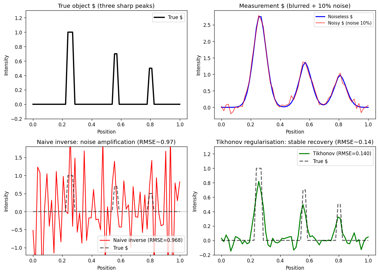
Top-left: the true 1-D object (three sharp peaks at positions 15, 35, 50). Top-right: the blurred+noisy measurement \(y = Hx + \epsilon\) (Gaussian blur, \(\sigma=3\) pixels, 10% noise). Bottom-left: naive least-squares inverse — RMSE ≈ 0.968, comparable to the signal amplitude, rendering the peaks indistinguishable from noise. Bottom-right: Tikhonov-regularised reconstruction (\(\lambda \approx 0.13\)) — RMSE ≈ 0.140, a 7× improvement. The peaks are correctly located but slightly broadened — the honest smoothing bias of regularisation.

• This is the most important figure in the lecture. Make sure students understand every panel before moving on.
• Panel 1 (true object): three sharp spikes at positions 15, 35, 50 with heights 1.0, 0.7, 0.5. These could represent atomic columns in a HAADF image.
• Panel 2 (measurement): the spikes have been blurred to broad humps by the Gaussian PSF. The noise (2% of signal) looks small in this panel — almost invisible.
• Panel 3 (naive inverse): RMSE≈0.968. The reconstruction is dominated by amplified noise — the true peaks at positions 15, 35, 50 are almost indistinguishable from the noise fluctuations. The 10% measurement noise was amplified roughly 10× (naïve RMSE / noise level ≈ 9.7×), consistent with the condition number κ≈230 and the limited noise floor suppression.
• Panel 4 (Tikhonov): RMSE≈0.140. The peaks are clearly visible and correctly located. The heights are slightly reduced from the true values (regularisation bias — the prior “pulls” the solution toward zero). The ratio naive/Tikhonov ≈ 7× — a genuine improvement. But the result is useful and interpretable, unlike the naive version.
• Key question to pose to students: “Is the Tikhonov result ‘correct’?” Answer: No, it is slightly wrong at every spike. But it is interpretably wrong — the error is bounded, the peaks are visible, and the bias is predictable. The naive result is uselessly wrong.

Why the naive inverse fails: the SVD picture (reference)

• Singular Value Decomposition of \(H\): \(H = U \Sigma V^T\) where \(\Sigma = \text{diag}(\sigma_1 \geq \sigma_2 \geq \ldots \geq \sigma_N)\).
• Naive inverse: \(\hat{x}_\text{naive} = V \Sigma^{-1} U^T y\) — divides by every singular value, including the tiny ones near zero.
• Tikhonov filter: \(\hat{x}_\lambda = V \, \widetilde{\Sigma} \, U^T y\) where \(\widetilde{\sigma}_i = \dfrac{\sigma_i}{\sigma_i^2 + \lambda}\) — replaces division by \(\sigma_i\) with a damped factor. (Formula shown as reference — not derived.)
• Intuition: the \(\lambda\) term adds a “floor” under each singular value before inversion. Small \(\sigma_i\) no longer blow up; large \(\sigma_i\) are barely affected (since \(\sigma_i^2 \gg \lambda\)).
• Every regulariser has a filter interpretation: L2 (Tikhonov) damps all singular values smoothly; L1 / TV acts as a non-linear filter that preserves edges.

• This slide presents the SVD formula as a reference only. The exam does NOT require students to derive it. They should understand the intuition: the \(\lambda\) floor prevents division by near-zero singular values.
• The Wiener filter in signal processing is essentially Tikhonov regularisation for convolution operators. If students know Wiener filters (e.g. from a signal-processing course), point out the connection.
• The generalised Tikhonov form \(\hat{x}_\lambda = (H^T H + \lambda L^T L)^{-1} H^T y\) allows more flexible regularisation: with \(L = I\) (identity), we get standard Tikhonov; with \(L = \nabla\) (gradient operator), we penalise rapid spatial variation; with \(L\) as the Laplacian, we penalise second-order roughness. All are special cases of the same SVD-filter picture.
• Transition: “Now that we know why the naive inverse fails, let us build the regularised framework.”

Regularisation: the core idea

• The variational formulation: instead of solving \(Hx = y\) directly, minimise a combined objective: \(\hat{x} = \arg\min_{x} \underbrace{\|Hx - y\|^2}_{\text{data fidelity}} + \lambda \underbrace{R(x)}_{\text{regulariser}}\) (shown as reference — not derived)
• Data fidelity: penalises solutions that do not fit the measurements. Large = “I don’t trust the reconstruction.”
• Regulariser \(R(x)\): penalises solutions that are “physically unreasonable.” Encodes our prior knowledge about the object.
• The weight \(\lambda\): controls the trade-off. Too small \(\lambda\): fits every noise fluctuation (overfitting). Too large \(\lambda\): ignores the data, returns the prior mean (underfitting).
• The Bayesian view (connection to Week 9): the data-fidelity term is the negative log-likelihood; the regulariser is the negative log-prior; minimising their sum = computing the MAP estimate. Bishop, Christopher M., (2006)

• The variational formulation is the central equation of the lecture. Show it prominently and make students copy it. It will reappear every time we discuss a specific regulariser.
• The three intuitions for \(\lambda\):
  1. \(\lambda = 0\): pure data fit → naive inverse → noise blow-up.
  2. \(\lambda = \infty\): pure prior → ignore the data → return the prior mean (e.g. a constant or zero image).
  3. Optimal \(\lambda\): the “Goldilocks zone” where data fit and prior are balanced.
• The Bayesian connection (Week 9): \(p(x \mid y) \propto p(y \mid x) p(x)\). Taking the log: \(\log p(x \mid y) = -\|Hx - y\|^2/(2\sigma_\epsilon^2) - R(x) + \text{const}\). The MAP estimate maximises this = minimises the combined objective. Different priors \(p(x)\) give different regularisers: Gaussian prior → L2 (Tikhonov); Laplace prior → L1; Markov random field → TV.
• “Regularisation encodes prior knowledge” is the single most important sentence. A student who understands this can derive any specific regulariser by asking: “what does this prior say about the object?”

The regularised objective: data + prior = stable reconstruction

• Data fidelity (left term): how well does the reconstruction fit the measurements?
  • Gaussian noise model → squared \(\ell_2\) residual: \(\|Hx - y\|_2^2\)
  • Poisson noise model (low-dose EELS/EDX) → Poisson negative log-likelihood
• Regulariser \(R(x)\) — the prior knowledge term:

Regulariser	Prior belief	Effect
\(\|x\|_2^2\) (L2)	Object values are small	Shrinks uniformly; smooth solutions
\(\|\nabla x\|_2^2\) (Tikhonov)	Object varies slowly	Suppresses oscillations; blurs edges
\(\|\nabla x\|_1\) (TV)	Object is piecewise constant	Preserves sharp edges
\(\|x\|_1\) (L1/sparsity)	Object is mostly zero	Compressed sensing: few non-zero atoms

• Choice of regulariser is a scientific choice, not just a mathematical one. TV is appropriate for HAADF images (atomic columns separated by vacuum); L2 is appropriate for smooth phase maps (STEM-ptychography potentials).

• The table is examinable: students should know what each regulariser assumes and what it produces.
• Poisson noise model detail: for low-dose EELS with \(\bar{n}\) expected counts, the log-likelihood term is \(\sum_i [\bar{n}_i(x) - y_i \log \bar{n}_i(x)]\) where \(\bar{n}_i(x) = (Hx)_i\). This replaces the squared residual in the low-dose regime. The combined objective is still minimised by gradient descent.
• TV vs L2 in practice: if the sample has sharp compositional boundaries (e.g. a core-shell nanoparticle), TV is much better — L2 will blur the boundary into a gradient. If the sample has smoothly varying composition (e.g. a diffuse interface), L2 is appropriate and TV will introduce staircase artefacts.
• Sparsity (L1): compressed sensing (Week 12 preview). If the object is sparse in some basis (e.g., few atomic columns against a dark background), L1 regularisation combined with a random measurement operator can reconstruct from far fewer measurements than a full scan — this is the mathematical basis of sparse 4D-STEM acquisition.

Building intuition: regularisation = taming the solution space

• Without regularisation: the solution space is infinite — every \(x\) with \(\|Hx - y\| \leq \|\epsilon\|\) is equally valid. The naive solver picks the one closest to zero in the least-squares sense, which happens to amplify noise catastrophically.
• With regularisation: we add a constraint surface \(\{x : R(x) \leq c\}\). The solution is the point where the data-fit ellipsoid first touches this surface.
• Geometric picture: L2 ball (\(\|x\|_2 \leq c\)) → solution lies in the interior → smooth, no sharp edges. L1 ball (\(\|x\|_1 \leq c\)) → solution tends to land at the corner of the diamond → sparse. TV ball → piecewise constant.
• EM intuition: “a physical STEM image cannot have arbitrary pixel-to-pixel oscillations.” The PSF of the probe physically limits the highest spatial frequency in the image — so any solution with higher-frequency components than the PSF is physically unreasonable. The regulariser enforces this.

• The geometric picture (solution ellipsoid touching the constraint ball) is the key intuition from Bishop Chapter 3. L1 corners promote sparsity; L2 circles do not. This is the same explanation as why LASSO sets some weights exactly to zero and Ridge does not.
• The EM physical argument is important: the PSF already limits the resolution. Asking for a reconstruction that is sharper than the PSF is physically nonsensical. The regulariser “knows” this; the naive inverse does not.
• Students often ask: “why not just truncate the SVD instead of using Tikhonov?” Truncated SVD (TSVD) is equivalent to setting all filter factors to 1 for \(\sigma_i > \tau\) and 0 otherwise — a hard threshold instead of a soft one. Tikhonov uses a soft threshold. Both are valid; Tikhonov is smoother and easier to differentiate.

Tikhonov (L2) regularisation

• Tikhonov regularisation adds an L2 penalty on the solution or its gradient: \(\hat{x}_\lambda = \arg\min_x \|Hx - y\|_2^2 + \lambda \|\nabla x\|_2^2\) Tikhonov, Andrey N. et al., (1977)
• For linear \(H\): the solution is analytic: \(\hat{x}_\lambda = (H^T H + \lambda \nabla^T \nabla)^{-1} H^T y\) (reference formula — no derivation required)
• What Tikhonov assumes: the object is spatially smooth — no sudden jumps in value. This is a Gaussian prior on the gradient: each pixel’s gradient is expected to be close to zero.
• Strengths: computationally cheap (one linear system solve); guaranteed unique solution; differentiable everywhere (smooth cost function, easy to optimise).
• Weaknesses: blurs sharp edges and boundaries. If the true object has sharp features (atomic columns, grain boundaries, interfaces), Tikhonov over-smooths them — a systematic bias that cannot be removed by tuning \(\lambda\).

• Tikhonov (1977) formalised the framework that had been used informally by many practitioners. His key insight: adding a penalty turns an ill-posed problem into a well-posed one, and the solution converges to the true solution as noise → 0 and λ → 0 (together, at the right rate).
• The gradient-penalised version (\(\lambda \|\nabla x\|_2^2\)) is sometimes called “second-order Tikhonov” or “Tikhonov-Philips” regularisation. The simpler \(\lambda \|x\|_2^2\) is sometimes called “zeroth-order Tikhonov” or just “Ridge” (in the ML sense).
• EM applications where Tikhonov works well: (1) phase maps from ptychography or differential phase contrast (the phase is expected to vary slowly across a uniform sample); (2) elemental maps from EDS when the composition varies smoothly (e.g. graded alloys).
• EM applications where Tikhonov fails: any sample with sharp interfaces (core-shell nanoparticles, grain boundaries, heterostructures). Use TV instead.

Total variation (TV) regularisation

• Total variation: \(\text{TV}(x) = \|\nabla x\|_1 = \sum_{i,j} \sqrt{(\partial_i x)^2 + (\partial_j x)^2}\) — the sum of gradient magnitudes over all pixels. Rudin, Leonid I. et al., (1992), doi:10.1016/0167-2789(92)90242-F
• What TV assumes: the object is piecewise constant — flat regions separated by sharp edges. This matches many EM specimens: uniform grains separated by narrow grain boundaries; atomic columns separated by vacuum.
• The key difference from L2: L1-norm on the gradient penalises large gradients but does NOT penalise a single step discontinuity — it costs exactly the step height, not its square. L2 penalises large gradients quadratically and therefore smears every boundary.
• Strengths: preserves sharp edges; very effective for HAADF STEM (atomic columns = local maxima) and tomographic reconstruction (dense particles in vacuum).
• Weaknesses: introduces “staircase artefacts” in smoothly varying regions; computationally more expensive than Tikhonov (non-differentiable at zero gradient — needs proximal operators or ADMM).

• Rudin, Osher and Fatemi (1992) introduced TV denoising for photographic images. It became the dominant regulariser for compressed-sensing tomography in the 2010s after Donoho and Candès showed that L1 minimisation recovers sparse signals from sub-Nyquist measurements.
• The staircase artefact: TV promotes piecewise-constant solutions. If the true object has a smooth gradient (e.g. a gradually changing composition), TV will represent it as a sequence of discrete flat steps — the “staircase.” This is a regularisation artefact that looks like structure but is not real. Always sanity-check reconstructions by asking whether smooth features show staircase behaviour.
• Proximal gradient descent for TV: the TV term is not differentiable at zero gradient, so standard gradient descent does not apply directly. Practical algorithms use the “proximal operator” of the TV norm (a local soft-thresholding of the gradient) interleaved with data-fidelity gradient steps. The ADMM (Alternating Direction Method of Multipliers) algorithm splits the problem into simpler sub-problems. Students do not need to implement these.
• Connection to Week 12: convolutional neural networks learned as denoisers (Plug-and-Play priors, DnCNN) replace the explicit TV term with a learned regulariser trained on millions of images. This is a more powerful prior but requires training data.

Tikhonov vs TV: comparison on a step-function signal

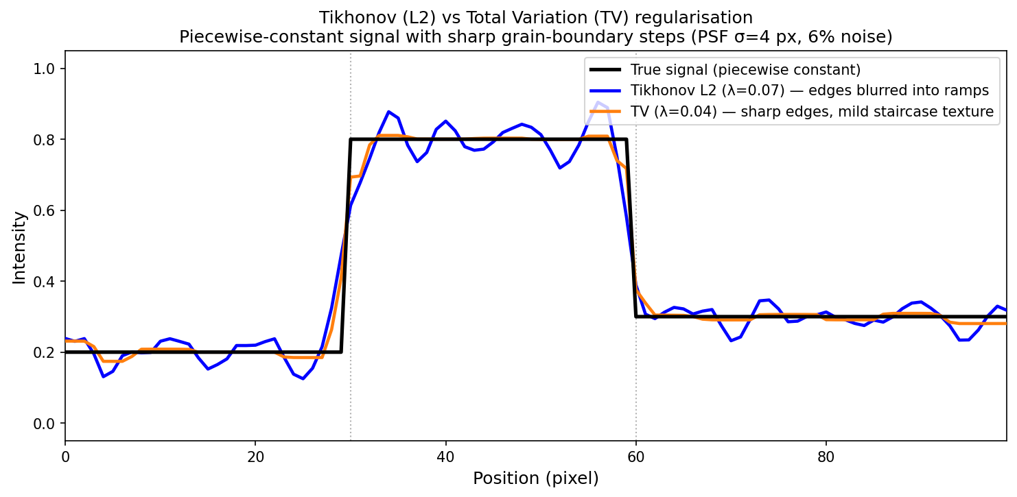
Comparison of L2 (Tikhonov) and total-variation (TV) regularisation on a 1-D piecewise-constant signal representing two grain-boundary steps (true values: 0.2 → 0.8 → 0.3; Gaussian PSF σ=4 px; 6% noise). Tikhonov (blue) blurs both transitions into broad ramps — the step positions are approximately correct but the edges are smoothed over several pixels. TV (orange) preserves the sharp step edges: the transitions are close to vertical, with only mild staircase texture in the flat regions. True signal in black (dashed vertical lines mark the step positions). TV RMSE ≈ 0.032; Tikhonov RMSE ≈ 0.057. Neither is perfect — the choice of regulariser determines which artefact appears.

• Walk through the three panels. The “truth” panel shows perfectly sharp step transitions at positions 30 and 55. This is what a HAADF image of a grain boundary might look like (projected along the boundary normal): a sharp step in column density.
• Tikhonov (blue): the transitions are visible but smeared over several pixels. The flat regions are well-reconstructed. The edge positions are slightly inaccurate (systematically inside the true boundary).
• TV (orange): the transitions are sharp and at approximately the correct positions. The flat regions show very slight staircase ripple.
• Key exam question: “Which regulariser should you use for a HAADF image of a grain boundary?” Answer: TV, because the grain boundary is a sharp edge and Tikhonov would smear it.
• Important honesty: both reconstructions have some artefact. The choice of regulariser cannot be separated from the choice of prior belief. If you believe the object is piecewise constant, use TV. If you believe it is smooth, use Tikhonov. Making the prior explicit makes the artefacts predictable.

Sensor fusion: HAADF + EELS as a regularised inverse problem

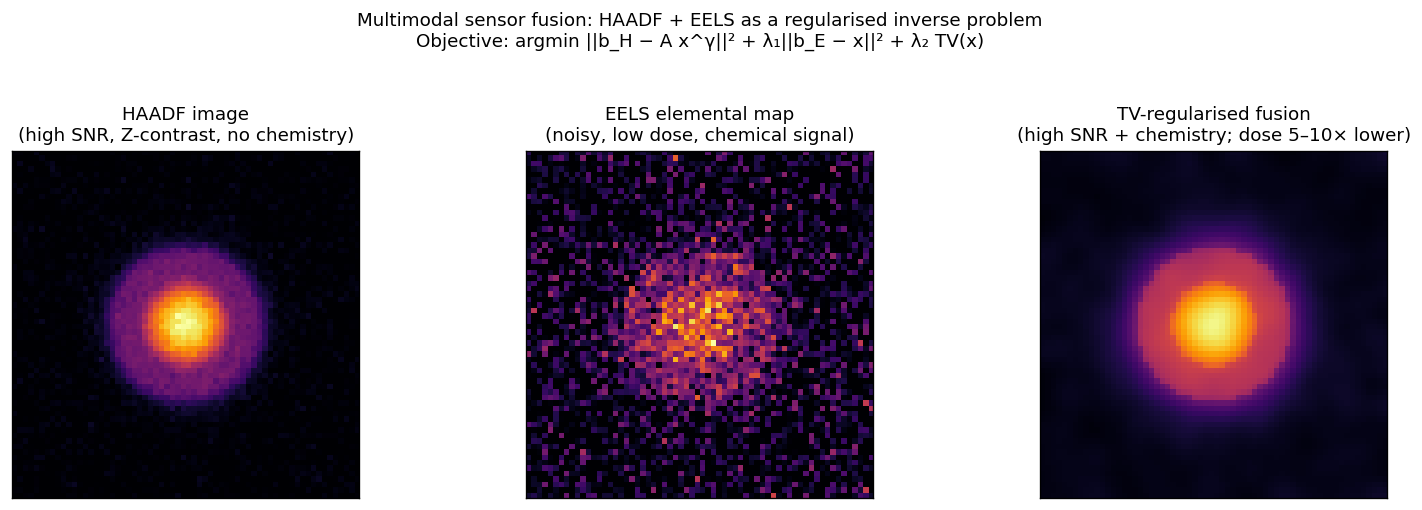
Three-panel comparison of a synthetic core-shell nanoparticle reconstruction. Left: HAADF image (high SNR, Z-contrast proportional to \(Z^{1.7}\), no chemical specificity). Centre: EELS elemental map (chemically specific but very noisy at low dose — 25% relative noise). Right: TV-regularised fusion result combining both signals, with objective \(\arg\min_{x \geq 0} \|b_H - Ax^\gamma\|^2 + \lambda_1 \|b_E - x\|^2 + \lambda_2\,\text{TV}(x)\) Pennycook, Stephen J. et al., (2012), doi:10.1007/978-1-4419-7200-2. The fused map recovers the core and shell structure with 5–10× dose reduction compared to a high-SNR EELS-only acquisition.

• Walk through all three panels. Left (HAADF): clear structure, bright core, dim shell. No way to tell which element is which — HAADF just measures total Z-contrast.
• Centre (EELS): the chemical signal is there but buried in noise. At the dose required to stay below beam-damage threshold, the SNR is too low to make a confident map.
• Right (fused): the structure from HAADF guides the noise suppression of the EELS signal. The TV regulariser ensures the elemental boundaries are sharp. The result is a high-quality chemical map at low dose.
• The objective function deconstruction: the first term (\(\|b_H - Ax^\gamma\|^2\)) ensures the chemical map is consistent with the HAADF Z-contrast (\(\gamma \approx 1.7\) is the HAADF exponent). The second term (\(\|b_E - x\|^2\)) ensures consistency with the EELS counts. TV(\(x\)) promotes sharp edges. The two λ values are the regularisation weights — both need tuning.
• Why is this “inverse problem” and not just “denoising”? Because we are fusing two different data modalities with different noise models and different forward operators (HAADF: non-linear Z-contrast; EELS: approximately linear in concentration). The combined objective has the same structure as any other regularised inversion.
• This is an active research area. Real implementations use ADMM or proximal gradient descent and report 300–500% SNR improvement at equal dose.

Choosing λ: the bias–variance trade-off

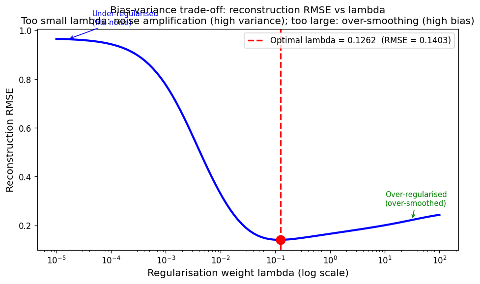
Reconstruction RMSE as a function of regularisation weight \(\lambda\) for the 1-D deblurring notebook (SEED=42, N=64, \(\sigma_\text{PSF}=3\), noise=10%). The curve has a clear U-shape: at \(\lambda=10^{-5}\) RMSE≈0.966 (under-regularised — fits noise); at \(\lambda=100\) RMSE≈0.243 (over-regularised — over-smoothed); minimum at \(\lambda^* \approx 0.126\) (red vertical line) with RMSE≈0.140. The optimal \(\lambda\) balances data fit against prior smoothness. This U-shaped RMSE curve is a genuine executed notebook result — reproduce it to verify your implementation.

• This figure is the notebook’s key diagnostic. Students must reproduce the U-shape with their own code (SEED=42).
• The U-shape is a universal feature of regularisation: it always exists when the model has enough capacity to overfit (low λ) and the regulariser imposes enough constraint to underfit (high λ). The location and depth of the minimum depend on the noise level, the forward operator, and the regulariser.
• Note that the optimal λ from the RMSE curve is not always accessible in practice: to compute RMSE you need the ground truth x_true, which you would not have with real EM data. That is why the L-curve (next section) exists — it estimates the optimal λ without needing the ground truth.
• The notebook reports (SEED=42): best λ≈0.126, best RMSE≈0.140, naive inverse RMSE≈0.968. Students should check their assert: naive_rmse > 4 * best_tikhonov_rmse — genuinely true (0.968 / 0.140 ≈ 6.9×).
• Transition: “When we don’t have ground truth — which is always the case with real EM data — how do we choose λ? The L-curve.”

Choosing \(\lambda\): the L-curve method

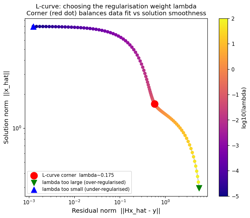
L-curve for the 1-D deblurring problem: horizontal axis = residual norm \(\|Hx̂ - y\|\) (data fit), vertical axis = solution norm \(\|x̂\|\) (solution complexity), both in log scale. Each point on the curve corresponds to a different \(\lambda\) (colour-mapped from blue = large \(\lambda\) to yellow = small \(\lambda\)). The curve has a characteristic L-shape. The corner (red dot, \(\lambda \approx 0.175\)) is the point of maximum curvature in log–log space — a data-only estimate of the optimal balance between data fit and solution norm. The L-curve corner (\(\lambda \approx 0.175\)) lies slightly above the true RMSE-optimal \(\lambda \approx 0.126\) (RMSE \(\approx 0.140\)): the L-curve is a heuristic, not an exact optimum. Blue triangle (bottom-right): small \(\lambda\) = under-regularised, very tight data fit but enormous solution norm. Green triangle (top-left): large \(\lambda\) = over-regularised, very small solution norm but poor data fit.

• The L-curve is a practical tool for choosing λ without ground truth. Walk through the shape: the vertical leg (top-left) represents over-regularised solutions — the data fit is poor but the solution is smooth. The horizontal leg (bottom-right) represents under-regularised solutions — the data fit is tight but the solution is noisy and large.
• The corner is the “Goldilocks point” where neither leg is unnecessarily extended. The curvature formula (radius of curvature in log–log space) finds this corner automatically.
• Note the difference between the L-curve corner λ≈0.175 and the true RMSE-optimal λ≈0.126 (RMSE≈0.140) from the notebook. They differ because the L-curve uses the solution norm ‖x̂‖ as a proxy for reconstruction quality — not the true error. The L-curve is a data-only heuristic — it does not require ground truth but is not always perfectly aligned with the RMSE minimum. This honest discrepancy (L-curve corner is ~1.4× larger than the RMSE-optimal λ) should be mentioned: the L-curve is a guide, not a guarantee. L-curve optimal λ≈0.175; RMSE-optimal λ≈0.126; best RMSE≈0.140.
• Other methods for choosing λ: (1) cross-validation (hold out a fraction of measurements, choose λ that minimises held-out residual); (2) Stein’s unbiased risk estimate (SURE) for Gaussian noise; (3) discrepancy principle (set λ so the residual matches the expected noise level ||ε||). All have pros and cons.
• Pacing: 3 minutes. The L-curve is a practical tool — spend time on the physical interpretation, not the curvature formula.

Practical \(\lambda\) selection: the discrepancy principle

• The discrepancy principle (Morozov, 1966): choose \(\lambda\) such that the residual matches the expected noise level. Criterion: \(\|H\hat{x}_\lambda - y\| \approx \|\epsilon\|\). This requires an estimate of the noise level — feasible if the noise model is known (Poisson: estimate from mean counts; Gaussian: estimate from blank-frame variance).
• Cross-validation (no noise model required): hold out a random subset of measurements; choose \(\lambda\) minimising the held-out residual. Computationally expensive for large problems.
• The L-curve (Hanson, 1992): maximise curvature in log-log plot of \(({\|H\hat{x}-y\|}, {\|\hat{x}\|})\) — no noise estimate needed, but can mis-estimate the optimal \(\lambda\) when the curve is nearly flat (ill-determined problems).
• In practice: start with the discrepancy principle if you know the noise level; use the L-curve as a sanity check; validate the chosen \(\lambda\) by visual inspection of the reconstruction (check for noise artefacts vs over-smoothing).

• The discrepancy principle is elegant but requires knowledge of the noise level. For Poisson-dominated EELS at N counts/pixel, the expected residual is \(\sqrt{N}\) (shot noise). For Gaussian noise at level σ, the expected residual is \(\sigma \sqrt{M}\) where M is the number of measurements.
• The main practical message: lambda selection is not automatic. It requires domain knowledge. A physicist who knows the noise level can use the discrepancy principle confidently. A data scientist without that knowledge should use cross-validation or the L-curve.
• Mentioning that ML-trained regularisers (Week 12) can learn the optimal denoising implicitly without λ selection — the prior is learned from training data and the “optimal λ” is absorbed into the network weights. This removes the λ-selection burden but introduces a new requirement: large labelled training datasets of (noisy input, clean target) pairs.
• Pacing: 2 minutes. This is a practical summary slide — do not over-explain.

\(\lambda\) selection in EM: what practitioners do

• Tomography: iterative SART with TV — start with \(\lambda = 10^{-2}\) and halve until the TV-regularised sinogram residual matches the estimated noise floor. Inspect the reconstruction visually: if edge ringing appears, increase \(\lambda\); if features are blurred, decrease \(\lambda\).
• EELS/EDX deconvolution: Fourier-ratio deconvolution with a Wiener filter (equivalent to Tikhonov in Fourier space). The Wiener parameter is chosen to match the SNR at each spatial frequency band.
• Sensor fusion (HAADF + EELS): typically set \(\lambda_\text{TV}\) by cross-validating on a held-out set of EELS spectra from a known reference area (e.g., the vacuum region has zero composition — the reconstruction should give zero there).
• Key lesson: there is no universal “correct” \(\lambda\). It depends on the noise level, the specimen, and the scientific question. Always report the \(\lambda\) used in publications — it is a hyperparameter of your measurement.

• The practical advice here is based on real workflow. For tomography: the TV regularisation weight is typically chosen by visual inspection after seeing the results at 3–5 values of λ. A log-scale sweep (λ = 0.001, 0.01, 0.1, 1.0) is standard.
• The Wiener filter reference: in Fourier-ratio deconvolution for EELS, the deconvolution multiplier at each spatial frequency \(k\) is \(H^*(k) / (|H(k)|^2 + \text{SNR}^{-1}(k))\) — exactly the Tikhonov filter with frequency-dependent λ given by the SNR. This is the most common form of regularised deconvolution in EELS.
• The “always report λ” point is a reproducibility argument. If you do not report λ, another lab cannot reproduce your deconvolution. λ is as fundamental a measurement parameter as the accelerating voltage or the camera length.
• Transition: “We have the theory. Let us apply it to electron tomography.”

Electron tomography: the forward model

• Goal: reconstruct the 3-D structure of a nanomaterial from a series of 2-D projection images collected at different tilt angles. Frank, Joachim, (2006), doi:10.1007/978-0-387-69008-7
• Forward model (Radon transform): each projection \(y_\theta(s) = \int_\text{ray} x(r)\, dl\) is a line integral of the 3-D density \(x\) along rays at tilt angle \(\theta\). For HAADF: \(x = Z^{1.7}\) weighted density; for BF: phase contrast; for EELS: elemental concentration.
• Collecting the tilt series: tilt the specimen in the TEM from \(-\theta_\text{max}\) to \(+\theta_\text{max}\) in steps of \(\Delta\theta \approx 1°\)–\(2°\). Record one image per tilt angle. Typical: 71 tilts at 2° increments (\(\pm70°\)), each at the same area.
• Dose management: total dose = dose per image × number of tilts. Beam-sensitive samples limit dose per image → fewer tilts → sparser Fourier coverage → more regularisation needed. This is the fundamental dose–quality trade-off in tomography.

• The Radon transform: R(x)(θ, s) = ∫∫ x(r, z) δ(r cos θ + z sin θ - s) dr dz. For parallel-beam geometry (common in TEM, unlike X-ray CT which uses fan-beam), the Fourier slice theorem applies exactly.
• Tilt step choice: 2° is a common default. Too small: many projections, high total dose, risk of beam damage. Too large: sparse Fourier coverage, missing-wedge-equivalent gaps between tilts. The Crowther criterion: for a particle of diameter d, the required number of tilts is π d / (2 Δx) where Δx is the pixel size. This gives ~60–90 tilts for a 50-nm nanoparticle at 1 nm/pixel.
• Bright-field vs HAADF for tomography: HAADF is preferred for tomography because it is approximately monotonic (thicker/heavier = brighter) — no contrast reversals with defocus. BF-TEM has diffraction contrast that can make thickness non-monotone, violating the Radon model.
• EELS tomography: requires 5-D data (x, y, tilt, energy) — each tilt is an EELS spectrum image. Enormously dose-intensive; requires very low dose per image and strong regularisation. Active research area.

Electron tomography: the missing wedge problem

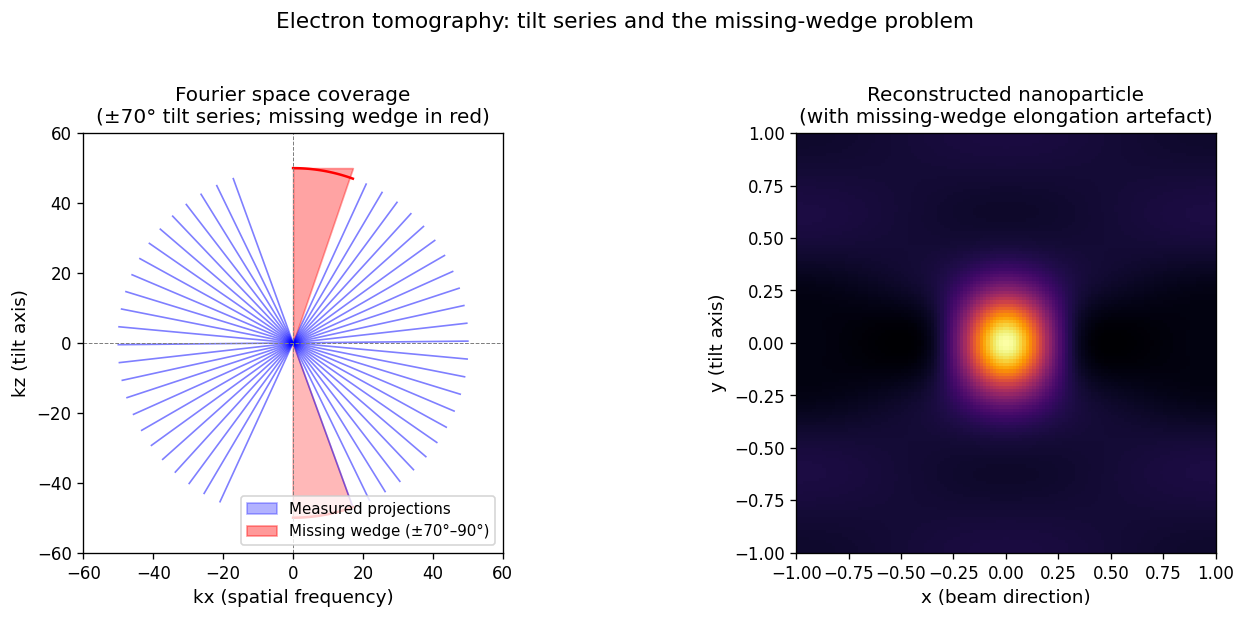
Fourier-space coverage for a ±70° tilt series (left): each blue line represents the 1-D slice measured by one projection. The red shaded region is the “missing wedge” — the angular sector from ±70° to ±90° that cannot be reached without mechanically shadowing the specimen holder. Right: reconstruction of a spherical nanoparticle with the missing-wedge artefact. The particle appears elongated in the beam direction (vertical) because the Fourier frequencies that encode vertical extent were never measured. This anisotropic elongation is not real structure — it is a missing-wedge artefact. Regular compressed-sensing methods Leary, Rowan et al., (2013), doi:10.1016/j.ultramic.2013.03.019 reduce but do not eliminate this artefact.

• The missing wedge is one of the most commonly misinterpreted artefacts in electron tomography. Inexperienced users see the elongation and think it represents real elongation of the particle. The diagnostic: (1) the elongation is always in the beam direction, not a sample-specific direction; (2) it is reproducible across all particles in the field of view; (3) it disappears (or shrinks) when the tilt range is extended.
• The 70° limit: most standard TEM holders allow ±70° maximum. Dedicated tomography holders with needle-like specimens allow ±80° or higher. Dual-tilt holders tilt around two orthogonal axes, which fills two orthogonal missing wedges at the cost of more complexity.
• Compressed sensing tomography: by using a sparse prior (L1 or TV), one can recover approximate 3D structure from even fewer tilts than the Crowther criterion requires. The trade-off: compressed sensing assumes the object has a sparse representation in some basis; artefacts appear when this assumption is wrong (e.g. a large amorphous region is not sparse).
• Resolution anisotropy: the resolution in the tilt plane is determined by the total angular range and the tilt step. The resolution out of the tilt plane is limited by the missing wedge. A good rule of thumb: resolution in the tilt plane ~ pixel size; resolution out of the plane ~ particle size / 2 for a ±70° tilt.

Tomographic reconstruction algorithms

• Filtered Back-Projection (FBP): analytical solution based on the inverse Radon transform. Fast (\(O(N^2 \log N)\)), but requires complete noiseless projections — poor performance with missing data or noise. Standard baseline algorithm.
• SART (Simultaneous Algebraic Reconstruction Technique): iterative method — alternates between forward projection (computing the synthetic sinogram from the current estimate) and back-projection (updating the estimate by distributing the residual back along rays). Slower than FBP but handles incomplete and noisy data gracefully.
• TV-SART (SART + TV regularisation): adds a TV denoising step after each SART iteration Saghi, Zineb et al., (2016), doi:10.1186/s40679-016-0020-3. Enforces piecewise-constant structure. State-of-the-art for nanoparticle tomography.
• Compressive sensing tomography: replaces SART with a direct L1 / TV minimisation Leary, Rowan et al., (2013), doi:10.1016/j.ultramic.2013.03.019. Can reconstruct from 10–20 tilts instead of 70 — a 5–7× dose reduction. Requires strong sparsity prior.

• FBP algorithm: (1) apply a ramp filter to each projection in Fourier space (compensates for the 1/r density of spokes in Fourier space); (2) back-project all filtered projections. Step 2 is the “smearing” step — each projection is spread back over the object space along the corresponding ray direction. The sum of all back-projections cancels the artefacts from step 2. With a perfect tilt series, the result is exact.
• Why FBP fails with missing data: the ramp filter assumes complete angular coverage. With a missing wedge, FBP introduces streaks and elongation artefacts that cannot be corrected post-hoc. SART handles missing data gracefully because it is iterative — it never uses the “missing” projections; it simply does not update the corresponding rows of the system matrix.
• SART update rule: x ← x + ω * H^+ (y - Hx) where H^+ is a scaled back-projector and ω is a relaxation parameter. One “cycle” processes all projections in sequence, applying one correction per projection. Convergence is guaranteed for 0 < ω < 2 / (spectral radius of H^+ H).
• TV-SART in practice: 50–200 SART iterations, each followed by a few steps of TV denoising (gradient descent on the TV term). The TV step size and the number of TV steps are additional hyperparameters. Standard values: λ_TV = 1e-2 to 1e-1; 3–5 TV steps per SART cycle.

Tomography in 3-D: an EELS spectroscopic example

• Challenge: 3-D elemental maps require a full tilt series of EELS spectrum images — 5-D data \((x, y, \theta, E)\) with extreme dose requirements.
• Breakthrough: Nicoletti et al. (2013) demonstrated 3-D spectroscopic tomography of silver nanocubes by EELS, mapping local surface plasmon resonances in 3D. Nicoletti, Osman et al., (2013), doi:10.1038/nature12469
• Method: 71-tilt HAADF + EELS spectrum-image series; TV-SART reconstruction on each energy channel; spatial resolution ~2 nm.
• Result: visualised the 3-D distribution of corner, edge, and face plasmon modes — modes that 2-D EELS cannot separate because they overlap in projection.
• What regularisation contributed: TV-SART allowed reconstruction from noisy EELS data (≪1 count/pixel in many energy channels) that would have been unusable with FBP.

• The Nicoletti 2013 Nature paper is one of the landmark results in electron tomography. It showed that EELS, despite its extremely low signal at each energy channel, can be regularised well enough to give 3-D spectroscopic maps with nm resolution.
• The surface plasmon story is beautiful physics: a silver nanocube has different plasmon modes at its corners, edges, and faces, each with a slightly different energy (detectable in EELS). In 2-D, these modes project on top of each other. In 3-D, they can be separated spatially. TV tomography made this measurement possible.
• Numbers: typical SNR for a single EELS tilt image ≈ 1–3. After TV tomographic reconstruction from 71 tilts: SNR improvement of ~√71 ≈ 8.4× (incoherent), further improved by TV denoising. Final 3-D SNR ≈ 10–25 — sufficient for structure identification.
• Mention this as a “worked example” of regularisation enabling a new measurement — not just improving an existing one. Without TV-SART, this measurement would have been physically impossible at tolerable dose.

Electron tomography: artefacts to be aware of

• Missing-wedge elongation: features elongated along the beam direction; severity scales with the missing angle. Diagnostic: elongation is always in beam direction, not specimen-specific.
• Streak artefacts (FBP): linear streaks between high-contrast features, radiating at the tilt angles with the largest spacing. Minimised by SART and TV regularisation.
• Over-regularisation artefacts: TV “staircase” in smoothly varying regions; Tikhonov blurring of sharp boundaries. Monitor residual \(\|Hx̂ - y\|\) — if it is much larger than the noise level, you are over-regularised.
• Dose damage artefacts: specimen changes during the tilt series. Manifests as phantom features that appear only in some tilts. Cannot be corrected by regularisation — must be minimised by reducing dose per image or using cryo-tomography.
• Honest reporting: every published tomogram must state the tilt range, tilt step, reconstruction algorithm, \(\lambda\) value (if regularised), and total dose. These are not optional metadata — they determine what artefacts may be present.

• Artefact awareness is as important as algorithm knowledge. A student who can run TV-SART but cannot identify its artefacts in the output is not ready for independent research.
• The “honest reporting” point is a reproducibility argument. The tilt range and λ are hyperparameters of the measurement, just like the accelerating voltage. Journals and reviewers are increasingly requiring these to be stated explicitly.
• Dose damage in cryo-tomography: the specimen is kept at liquid-nitrogen temperature to reduce beam-induced movement. Even so, radiation damage accumulates over the tilt series. Some labs use dose-symmetric tilt schemes (collect the most critical central tilts at low accumulated dose, add extreme tilts later) to minimise damage to the most informative data.
• Challenge question for students: “If a TV-regularised tomogram shows a very sharp boundary between two phases, how would you determine if it is real or a TV staircase artefact?” Answer: (1) compare with a mildly Tikhonov-regularised reconstruction — if both show the boundary, it is real; (2) check the raw HAADF images at the relevant tilts — is the boundary visible even in the projections?

Dose reduction through sensor fusion: the SNR argument

• The dose-quality dilemma: EELS is dose-limited. At beam-damage-safe dose (e.g. \(10^5\) e⁻/nm² for most oxides), typical EELS counts per pixel per eV are 10–100 — SNR ≈ 3–10. Standard EELS maps at this dose are too noisy to interpret.
• The brute-force solution: increase dose by 10× → SNR improves by \(\sqrt{10} \approx 3.2\times\), but beam damage destroys the specimen.
• The smart solution (fusion): HAADF provides a structural prior for free (it requires negligible extra dose). The HAADF prior constrains where atomic columns are, dramatically reducing the effective noise in the EELS map.
• Dose budget equation: fusion achieves the SNR of \(D_\text{HAADF} + 10 D_\text{EELS}\) with only \(D_\text{HAADF} + D_\text{EELS}\) dose. In practice: 5–10× dose reduction for equivalent chemical map quality. Pennycook, Stephen J. et al., (2012), doi:10.1007/978-1-4419-7200-2
• Why this is not “cheating”: the prior is applied only where HAADF structure is trusted. If HAADF shows a boundary, the EELS map is allowed to be sharp there. If HAADF is flat, the EELS map is smoothed. The prior is conditional on the data, not imposed unconditionally.

• The “smart solution” framing is important: we are not using the HAADF data to fabricate EELS information. We are using it to suppress noise in the EELS data where the HAADF structure supports the inference.
• The dose budget equation analogy: think of HAADF structural information as “borrowed information.” The HAADF tells us where atomic columns are (structural framework). The EELS tells us what those columns are made of (chemical detail). Together they determine the full picture with less dose than either alone.
• Warning about the “not cheating” point: if the HAADF structure is wrong (e.g. due to channelling artefacts or probe broadening in thick specimens), the fusion will transfer those errors into the EELS map. Always validate fusion results against raw EELS data on thin reference areas.
• 5–10× dose reduction: this is a literature claim from several papers demonstrating HAADF-guided EELS denoising. The exact factor depends on the specimen, the SNR ratio between modalities, and the TV weight.

Multimodal sensor fusion: why fuse HAADF + EELS?

• HAADF alone: high SNR (thousands of counts/pixel), high spatial resolution (≤ 1 Å), but only proportional to \(Z^{1.7}\) — cannot distinguish elements with similar Z (e.g. Fe vs Co vs Ni).
• EELS/EDX alone: chemically specific (distinguishes every element), but noisy (10–100 counts/channel at safe dose) — spatial resolution limited by SNR, not by the probe.
• The fusion idea: HAADF gives us structural geometry; EELS/EDX gives us chemistry. Fusing them: use HAADF as a structural prior to guide EELS noise suppression, reducing required dose by 5–10×. Pennycook, Stephen J. et al., (2012), doi:10.1007/978-1-4419-7200-2
• This is a regularised inverse problem: \(\hat{x} = \arg\min_{x \geq 0} \underbrace{\|b_H - Ax^\gamma\|^2}_{\text{HAADF consistency}} + \lambda_1 \underbrace{\|b_E - x\|^2}_{\text{EELS fidelity}} + \lambda_2 \underbrace{\text{TV}(x)}_{\text{edge prior}}\) (reference formula)
• First term: the HAADF signal constrains the structural envelope — the fused elemental map must explain the observed Z-contrast.

• The HAADF exponent γ ≈ 1.7: in the incoherent approximation, the HAADF signal at column position r is proportional to ∫ Z(r)^1.7 dz where the integral is along the beam direction. This is not the exact quantum-mechanical cross-section, but a good approximation for qualitative use. For quantitative Z-contrast, the correct exponent must be calibrated against known standards.
• Why EELS is dose-limited: EELS measures the energy lost by a transmitted electron when it excites a core-level electron (K, L, M edges). The core-loss cross-section is much smaller than the elastic scattering cross-section. At safe dose (~10^5 electrons/nm² for most oxides), a typical EELS count rate is 10–100 counts per pixel per eV — very noisy.
• The two λ parameters: λ₁ controls how much weight to give the EELS data relative to the HAADF constraint; λ₂ controls the TV edge sharpness. In practice, λ₁ is often set small (EELS is trusted less than HAADF), and λ₂ is set to match the HAADF edge sharpness.
• Results from the literature: TV-regularised HAADF+EELS fusion has been demonstrated to reduce required EELS dose by 5–10× while maintaining chemical accuracy at ~5% relative error on elemental fractions. Reference: several papers from the Midgley group at Cambridge.

The fusion objective: a term-by-term breakdown

• Term 1 — HAADF consistency: \(\|b_H - Ax^\gamma\|^2\) where \(A\) is the PSF-convolution operator, \(b_H\) is the measured HAADF image, and \(\gamma \approx 1.7\). This term uses the high-SNR HAADF data to constrain the total scattering power (= \(Z\)-contrast envelope) of the elemental map.
• Term 2 — EELS/EDX fidelity: \(\|b_E - x\|^2\) (for Gaussian noise) or \(\sum_i [x_i - b_{E,i} \log x_i]\) (Poisson model, better for low counts). This term ensures the fused map agrees with the chemically specific but noisy spectroscopic signal.
• Term 3 — TV regulariser: \(\text{TV}(x) = \|\nabla x\|_1\). The structural prior: the elemental map is piecewise constant (consistent with atomic-resolution HAADF showing discrete columns).
• Constraint \(x \geq 0\): elemental concentrations cannot be negative — a physical non-negativity constraint that eliminates unphysical solutions and stabilises the optimisation.
• Optimisation: solved by ADMM or proximal gradient descent; typical runtime 10–60 s on a modern GPU for a 256×256 map.

• The non-negativity constraint \(x \geq 0\) is subtle but important. Without it, the optimiser can produce negative concentrations as a numerical artefact. With it, the projected gradient step forces the solution to stay in the positive orthant.
• ADMM overview (not examinable): the key idea is to introduce auxiliary variables to split the non-smooth TV term from the smooth data terms. Each sub-problem has a closed-form or efficiently solvable update. The algorithm alternates between sub-problems until convergence. Students do not need to implement ADMM — they need to understand that it exists and why it is needed (TV is not differentiable at zero gradient).
• Practical implementation note: in the sensor_fusion.qmd source material, the Poisson model for EELS is used explicitly (the log term). This is important for low-dose EELS where Gaussian MSE would underweight noisy channels. Using the correct noise model is as important as choosing the regulariser.
• The non-negativity + Poisson + TV combination is known as the “Poisson TV” problem. Its proximal operator has been well studied. Several open-source packages implement it (HyperSpy, ASTRA toolbox, scikit-image restoration).

HAADF + EELS fusion: the reconstruction result

Sensor fusion result for a synthetic core-shell nanoparticle. Left: HAADF image (high SNR, Z-contrast — structure visible, no chemistry). Centre: EELS elemental map at low dose (chemically specific but signal buried in 25%-relative noise). Right: TV-regularised fusion, minimising \(\|b_H - Ax^\gamma\|^2 + \lambda_1\|b_E - x\|^2 + \lambda_2\,\text{TV}(x)\). The core (bright) and shell (dim ring) are clearly distinguished in the fused map — the HAADF structural prior guided noise suppression without requiring the full EELS dose. Honest caveat: the reconstruction sharpens edges but may slightly over-estimate core-shell contrast (TV over-sharpening artefact) at high \(\lambda_2\).

• This slide repeats the fusion figure to emphasise the “result” rather than the “method.” The earlier slide introduced the objective; this one focuses on what students should observe.
• The honest caveat about TV over-sharpening: TV can over-enhance edges, making a gradual diffuse interface look sharper than it really is. To check: look at the raw HAADF — does it show the same sharpness? If HAADF shows a gradual edge but the fused EELS map shows a sharp step, the TV has over-regularised.
• Practical assessment: for a real experiment, compare (a) the raw EELS map after standard background subtraction; (b) the PCA-denoised EELS map (Week 8); (c) the TV-fused map. Each should be more useful than the last. If the TV-fused map differs wildly from the PCA-denoised version, investigate whether the HAADF prior is pulling the EELS toward structure-correlated noise.
• The 5–10× dose reduction claim: if the raw EELS map requires 10× more dose to achieve acceptable SNR compared to HAADF, and the fused approach achieves the same SNR with HAADF dose + 0.1× EELS dose, the total dose reduction is ~10×. This is the practical motivation for developing these methods.

Fusion as the general framework: from deblurring to multi-modal reconstruction

• Every EM reconstruction problem fits the same template: \(\hat{x} = \arg\min_x \sum_k \lambda_k \text{DataFidelity}_k(x, y_k, H_k) + \lambda_\text{reg} R(x)\)
• Different modalities = different forward operators \(H_k\):
  • HAADF: $H_k = $ PSF convolution + \(Z^{1.7}\) nonlinearity
  • EELS: $H_k = $ PSF convolution (approximately linear in concentration)
  • EELS tomography: $H_k = $ Radon transform + PSF
  • 4D-STEM ptychography (Week 12): $H_k = $ electron scattering simulation (nonlinear)
• The framework is modular: add a new modality by adding a new data-fidelity term with the corresponding forward operator and noise model. The regulariser \(R(x)\) stays the same.
• The limit of the framework: if \(H_k\) is highly nonlinear or not differentiable, the optimisation becomes much harder — this motivates neural-network-based inversion (Week 12).

• The “modular” framing is important for students thinking about their own projects. If they need to combine HAADF + EDS + EELS + BF images of the same sample, they can write down one combined objective with four data-fidelity terms and one regulariser. The optimisation will be challenging but the framework is clear.
• The “same framework” argument connects back to Week 4 (regularised regression = forward model + L2 regulariser), Week 8 (autoencoder loss = reconstruction loss + bottleneck constraint), Week 9 (GP posterior = data likelihood + prior). All of these are special cases of the same Bayesian MAP framework.
• Nonlinear forward operators: 4D-STEM ptychography requires computing the multislice electron propagation through the specimen — an expensive, nonlinear forward model. This makes the optimisation non-convex and much harder. Neural networks (learned regularisers) can handle this because they can be trained end-to-end without requiring differentiability of the forward operator.
• Pacing: 2 minutes. This is a synthesis slide — emphasise the “one framework, many modalities” message.

What good reconstruction looks like — and its honest limits

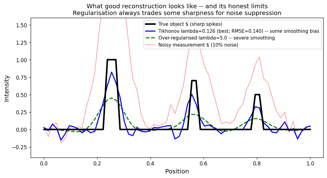
Reconstruction quality comparison for the 1-D deblurring notebook (SEED=42, noise=10%). Black curve: true object (three sharp spikes). Red curve: noisy measurement \(y\). Blue curve: Tikhonov at near-optimal \(\lambda \approx 0.126\) (RMSE ≈ 0.140) — peaks correctly located, heights slightly underestimated (regularisation bias). Dashed green curve: over-regularised Tikhonov (\(\lambda = 5.0\), RMSE ≈ 0.189) — peaks smeared into a broad hump. The best achievable reconstruction is not “perfect” — regularisation always trades some sharpness for stability. The naive inverse (RMSE ≈ 0.968, not shown) is dominated by noise and useless.

• This slide is the honest summary of the lecture. The best Tikhonov reconstruction is not “correct” — it is just the least wrong among all stable solutions. The peaks are found, but their heights are slightly reduced and their positions are slightly displaced.
• The phrase “regularisation always trades some resolution for stability” should be written on the board. It is a fundamental limit of any inverse problem, not a limitation of a particular algorithm. To get better resolution, one needs more informative measurements (higher SNR, more tilts, wider PSF bandwidth) — not a better algorithm applied to the same data.
• The over-regularised case (\(\lambda = 5.0\)) is shown to illustrate how easy it is to accidentally over-regularise. If \(\lambda\) is set too large (as often happens when practitioners use “safe” large values), multiple features merge into one and the reconstruction is qualitatively misleading. This is worse than a noisy reconstruction because it looks clean and authoritative.
• Key message: “A reconstruction that looks clean is not necessarily correct. Always cross-check with the raw data. If the residual \(\|Hx̂ - y\|\) is much larger than the noise level, you are over-regularised and your reconstruction is biased.”

Reconstruction limits: what we cannot recover

• Null space of \(H\): all information in the null space of the forward operator \(H\) is irreversibly lost. No algorithm can recover it from \(y\) — not even perfect regularisation.
  • Tomography: Fourier frequencies in the missing wedge. The corresponding structural features are gone.
  • Deblurring: spatial frequencies where the PSF’s OTF is effectively zero (below the noise floor). Deconvolution cannot recover these — it can only interpolate consistently.
• Noise floor limit: reconstruction accuracy is bounded by \(\|\epsilon\| / \sigma_\text{min}(H)\). Better SNR (more dose, longer acquisition) raises the floor — not better algorithms.
• Regularisation bias: the prior always biases the solution toward the prior’s mode. If the prior is wrong (e.g., TV prior on a smoothly varying sample), the bias is systematic and misleading.
• Practical diagnostic: plot the normalised power spectral density of the reconstruction. If it drops below the noise floor at some frequency, that frequency was not recovered — it was filled by the prior.

• The null space concept is the deepest point in the lecture. Encourage students to think carefully: “What information did the measurement operator destroy?” For tomography: the missing-wedge frequencies. For deblurring: the high-frequency components where the OTF is near zero.
• The noise floor formula: the smallest recoverable signal is determined by the smallest singular value and the noise level. With κ=230 and 1% noise: δx ≥ 0.01 * κ = 2.3 — worse than the signal! With Tikhonov regularisation, the effective condition number is reduced to κ_eff = σ_max / sqrt(λ), which for λ=0.013 gives ~√(σ_max²/λ) ≈ manageable.
• Practical power spectral density diagnostic: plot the radially averaged power spectrum of the reconstruction vs the reconstruction noise floor. If the spectrum drops to the noise floor at some frequency k_max, you can only trust spatial features larger than 1/k_max. This is the resolution limit of the reconstruction.
• Honest note to give students: “If a published reconstruction shows features sharper than the PSF of the instrument, be sceptical. Either the forward model was wrong, or the reconstruction algorithm was over-claiming.”

Limits, open problems, and forward link to Week 12

• What Week 11 gives you: the complete classical toolbox — forward model \(y = Hx + \epsilon\), ill-posedness (non-uniqueness + noise amplification), regularisation (Tikhonov + TV), \(\lambda\) selection (L-curve + discrepancy), tomography (SART + missing wedge), and sensor fusion (HAADF + EELS).
• What it cannot do: (1) highly nonlinear forward operators (e.g. multislice electron scattering in ptychography); (2) extremely limited measurements (< 10 tilt angles, single shot); (3) learning the prior from data (the regulariser is hand-crafted, not learned).
• Week 12 — Imaging inverse problems II: ptychography (a phase-retrieval inverse problem with a nonlinear forward model), generative priors (deep networks as learned regularisers), and physics-informed neural networks (PINN-based inversion). Same framework, more powerful priors.
• The three-week arc (Weeks 9–11): calibrated uncertainty (GP) → intelligent acquisition (BO/RL) → stable reconstruction (inverse problems). Together, these form the complete data-science loop for quantitative EM.

• Close the arc explicitly. Students who have followed all three weeks should see a coherent story: (1) the GP tells us where uncertainty is large → (2) active acquisition measures at high-uncertainty/high-value locations → (3) inverse problems reconstruct the physical quantity from those measurements. The full pipeline: sense → plan → reconstruct → update GP → sense again.
• The “highly nonlinear forward operators” point is important for Week 12 motivation. Electron scattering in a thick specimen requires solving the Schrödinger equation at each slice — the forward model is a multiply differentiable function, not a simple matrix. Classical gradient-based inversion (like SART) becomes very expensive. Neural networks that are trained end-to-end on (simulated measurement, ground truth) pairs can effectively learn an approximate inverse directly.
• The “learned regulariser” concept: instead of writing down TV or Tikhonov, train a CNN denoiser on a large dataset of (noisy image, clean image) pairs. Plug this denoiser into the ADMM framework as the proximal operator. This is “Plug-and-Play” (PnP) regularisation — the topic of the Kamilov review paper cited in this deck.
• Final pacing: 3 minutes. Leave 2 minutes for questions before ending.

Continue

• → Next: Week 12 — Imaging inverse problems II
• ← Back: Week 10 — Active & automated electron microscopy
• All courses

References

A plug-and-play image reconstruction framework, IEEE Signal Processing Magazine, Ulugbek S. Kamilov, Charles A. Bouman, Gregery T. Buzzard, & Brendt Wohlberg https://doi.org/10.1109/MSP.2022.3199595.

Sur les problèmes aux dérivées partielles et leur signification physique, Jacques Hadamard.

Electron tomography: Methods for three-dimensional visualization of structures in the cell, Joachim Frank https://doi.org/10.1007/978-0-387-69008-7.

Compressed sensing electron tomography, Ultramicroscopy, Rowan Leary, Zineb Saghi, Paul A. Midgley, & David J. Holland https://doi.org/10.1016/j.ultramic.2013.03.019.

Reduced-dose and high-speed acquisition strategies for multi-dimensional electron microscopy, Advanced Structural and Chemical Imaging, Zineb Saghi, Rowan Leary, David J. Holland, & Paul A. Midgley https://doi.org/10.1186/s40679-016-0020-3.

Pattern recognition and machine learning, Christopher M. Bishop.

Solutions of ill-posed problems, Andrey N. Tikhonov & Vasiliy Y. Arsenin.

Nonlinear total variation based noise removal algorithms, Physica D: Nonlinear Phenomena, Leonid I. Rudin, Stanley Osher, & Emad Fatemi https://doi.org/10.1016/0167-2789(92)90242-F.

Scanning transmission electron microscopy: Imaging and analysis, Stephen J. Pennycook & Peter D. Nellist https://doi.org/10.1007/978-1-4419-7200-2.

Three-dimensional imaging of localized surface plasmon resonances of metal nanoparticles, Nature, Osman Nicoletti, Francisco de la Peña, Rowan K. Leary, David J. Holland, Caterina Ducati, & Paul A. Midgley https://doi.org/10.1038/nature12469.