Materials Genomics
Unit 9: Neural Networks for Materials Properties
FAU Erlangen-Nürnberg


§0 · Frame
01. Today’s Question
What does a neural network for an atomic system look like?
- A crystal is not a vector and not an image.
- It is a graph of atoms under periodic boundary conditions, with a precise set of symmetries.
- A generic MLP on a Magpie vector is blind to most of that structure.
- Today: the architectures designed to respect atomic-system geometry.
What this unit is not.
- Not a re-introduction of the neuron, MLP, backprop, or convolution — that is MFML W4.
- Not an attention / transformer derivation — that is MFML W10, forward-linked here in §G.
- Not a re-derivation of crystal graphs — that is MG U7, recapped in one slide.
- Not a re-derivation of local environments — that is MG U6, recapped in one slide.
02. Where We Are
Recap — what we already have
- MFML W4: the neuron, MLP, backprop, convolutions (Goodfellow et al. 2016).
- MFML W10 (preview): attention and transformers — forward-linked in §G.
- ML-PC W4: neuron-level NN with materials-imaging examples.
- MG U6: local atomic environments, SOAP, ACSF.
- MG U7: crystals as graphs under PBC (Sandfeld et al. 2024).
- MG U8: benchmark discipline — grouped splits, residual analysis.
Today — Unit 9 in one line
- Compose MFML’s NN primitives with MG’s structural representations to build neural networks on atomic systems.
- Eight sections: recap, why-generic-fails, SchNet, CGCNN, MEGNet/ALIGNN/M3GNet, equivariance, transformers + foundation models, wrap-up.
03. Learning Outcomes
By the end of 90 minutes, you can:
- Explain why a generic MLP is the wrong model class for an atomic system, and name the four symmetries that must be respected.
- Describe SchNet’s continuous-filter convolution and why a discrete kernel is inadequate for atoms.
- Implement, conceptually, a CGCNN message-passing step on a crystal graph and connect it to MG U7.
- Place MEGNet, ALIGNN, M3GNet in the atom–bond–angle hierarchy and identify which target each is best for.
- Explain why E(3)-equivariance matters for forces and name the NequIP / Allegro / MACE family.
- Describe the role of transformer-style attention and foundation models (Matformer, OMat24, GNoME) for materials in 2024–2026.
- Choose an architecture for a given problem based on dataset size, target type, and physics constraint.
- Articulate the bridge to Unit 10: foundation-model embeddings as the central object of representation learning.
§A · Context recap
04. NN basics from MFML W4 — what we are not re-deriving
Assumed primitives
- Neuron: \(y = \sigma(\mathbf{w}^\top \mathbf{x} + b)\).
- MLP: stacked neurons; universal approximator under mild conditions (Goodfellow et al. 2016).
- Backprop: gradient via chain rule on a differentiable loss.
- Convolution: translation-equivariant linear map on a regular grid.
Why “regular grid” is the catch today
- Convolutions exploit translation on a grid: pixel \((i, j)\) + offset \((u, v) \to\) pixel \((i+u, j+v)\).
- An atom at position \(\mathbf{r}_i\) has no grid neighbour at fixed offsets.
- Two oxygens 2.3 Å apart and 2.7 Å apart need different kernels — but a discrete CNN has no slot for either.
- This is the central reason atomic-system NNs need a different convolution.
05. Crystals as graphs (recap from MG U7)
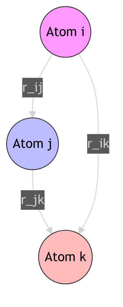
The graph encoding
- Nodes: atoms with chemistry features (\(Z\), oxidation state, electronegativity).
- Edges: neighbour relationships under PBC, found by a cutoff radius or k-nearest-neighbours search across periodic images.
- Edge attributes: interatomic distances \(r_{ij}\), optionally angles or bond types.
- Global state (optional): crystal system, density, temperature.
MG U7 contract still holds today. PBC are enforced at graph-construction time; cutoff and RBF parameters are documented; reproducibility starts with a deterministic graph.
06. Local atomic environments (recap from MG U6)
The MG U6 picture
- A property of a material often depends on local motifs: coordination, bond lengths, bond angles, elemental neighbourhoods.
- MG U6 introduced fixed local descriptors: SOAP, ACSF, Voronoi statistics — invariant by construction, hand-engineered.
- Pooled into a material-level vector for downstream regression.
Today’s question
- What if the network learns the local descriptor itself, end-to-end with the predictor?
- That is exactly what a message-passing layer does: each atom’s hidden state \(\mathbf{v}_i^{(t)}\) at layer \(t\) is a learned descriptor of its \(t\)-hop environment.
- SOAP/ACSF were hand-crafted; SchNet/CGCNN/ALIGNN are learned.
§B · Why generic NNs are not enough for atomic systems
07. The MLP-on-Magpie failure
Setup
- Input: Magpie vector \(\mathbf{x} \in \mathbb{R}^{132}\) — pooled elemental statistics from a chemical formula.
- Model: MLP with two hidden layers.
- Target: band gap, formation energy, etc.
- This is a strong, common baseline (MG U6 / U8).
The failure mode
- The Magpie vector depends only on composition.
- Two polymorphs with the same composition but different crystal structures map to the same input — and therefore the same prediction.
- Cubic vs hexagonal? Diamond vs graphite? Identical Magpie vector.
- For motif-sensitive properties (band gap, modulus, conductivity), this is a structural blind spot.
08. The four symmetries we must respect
The four physical symmetries of an atomic-system property
- Translation: \(f(\{\mathbf{r}_i + \mathbf{t}\}) = f(\{\mathbf{r}_i\})\).
- Rotation: \(f(\{R\mathbf{r}_i\}) = f(\{\mathbf{r}_i\})\) for invariant scalars; equivariant transform for vectors/tensors.
- Permutation: \(f(\pi(\{\mathbf{r}_i\})) = f(\{\mathbf{r}_i\})\) — atom labels are arbitrary.
- Periodicity: \(f\) is invariant under cell translation by lattice vectors.
Two ways to handle a symmetry
- Bake it in (architectural): the network is exactly invariant by construction. Cost: design constraint. Benefit: zero data spent learning the symmetry.
- Learn it (data-augmentation): rotate the inputs, retrain. Cost: much more data. Benefit: none for materials, where data is scarce.
09. Invariance vs equivariance
Scalar property: invariance
- \(f(R \cdot \text{input}) = f(\text{input})\).
- Examples: total energy \(E\), formation energy, band gap, bulk modulus.
- Implementation: build the network from rotationally invariant inputs (distances, angles, scalars).
Vector / tensor property: equivariance
- \(f(R \cdot \text{input}) = R \cdot f(\text{input})\).
- Examples: forces \(\mathbf{F}_i = -\partial E / \partial \mathbf{r}_i\), dipole moments, stress tensor.
- Implementation: carry vector / tensor features through the layers, with strict equivariance constraints.
Cardinal rule. A scalar-only architecture can produce forces — via autograd through the energy. A vector-only architecture can produce energies — via an invariant readout. But mixing the two carelessly breaks physics.
10. The symmetry group E(3) / SE(3)
E(3): the Euclidean group in 3D
- Translations \(\mathbf{t} \in \mathbb{R}^3\).
- Rotations \(R \in O(3)\) (including reflections).
- E(3) = translations \(\rtimes\) O(3).
SE(3): orientation-preserving subgroup
- Translations \(\mathbf{t} \in \mathbb{R}^3\).
- Rotations \(R \in SO(3)\) (no reflections).
- SE(3) = translations \(\rtimes\) SO(3).
Why this matters for materials
- Most properties are invariant under SE(3): rotation alone leaves them unchanged.
- Chiral materials (some spirals, twisted heterostructures) are not invariant under reflection — those need SE(3), not full E(3).
- Modern equivariant networks (§F) are precisely E(3)- or SE(3)-equivariant, with the choice driven by the physics.
E(3) is not the whole story for crystals. A good atomic ML model respects E(3)/SE(3) plus permutation plus periodicity. Papers say “E(3)-equivariant” because rotation/translation are the hard part architecturally; permutation and PBC are handled separately (slides 11+).
11. Permutation invariance and PBC inside the network
Permutation invariance via aggregation
- The hidden representation of atom \(i\) is updated by aggregating messages from its neighbours: \[ \mathbf{v}_i^{(t+1)} = U^{(t)}\!\left( \mathbf{v}_i^{(t)},\; \bigoplus_{j \in N(i)} \mathbf{m}_{ij}^{(t)} \right) \]
- \(\bigoplus\) is sum / mean / max — symmetric under permutation of \(N(i)\).
- Stacking layers preserves permutation invariance.
PBC at graph-construction time
- Build the neighbour list across periodic images of the cell.
- Edges encode displacement vectors \(\mathbf{r}_{ij}\) that may span image boundaries.
- The network sees only the graph; PBC are inherited automatically.
- Common bug: forget to enumerate periodic images \(\to\) disconnected graphs \(\to\) wrong predictions on the cell boundary.
§C · SchNet and continuous-filter convolutions
12. The SchNet idea
Setting (Schütt et al. 2017, 2018)
- Input: a molecule — a set of atoms \(\{Z_i, \mathbf{r}_i\}_{i=1}^N\) in 3D.
- Goal: predict total energy \(E\) (and, via autograd, forces).
- Constraint: invariance under translation, rotation, and permutation; no hand-crafted descriptors.
The central object: a continuous-filter convolution
- Atoms are not on a grid \(\to\) no discrete kernel.
- Replace the discrete kernel with a function \(W(r)\) — itself a small neural network of the interatomic distance \(r\).
- Evaluate \(W\) at the actual \(r_{ij}\) of each pair.
- This is the prototype “neural network on atoms.”
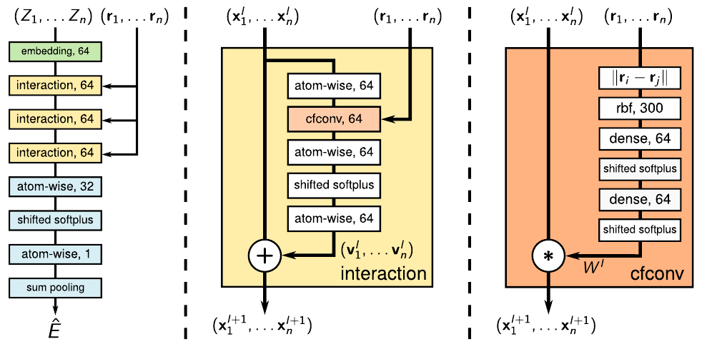
SchNet architecture (Schütt et al. 2017): atom embedding \(\to\) interaction blocks (cfconv) \(\to\) atom-wise MLP \(\to\) sum readout \(\hat{E}\).
13. Why a continuous filter
The discrete-CNN obstruction
- A 2D CNN kernel has slots at fixed offsets: \((\Delta x, \Delta y) \in \{-1, 0, +1\}^2\).
- For atoms, no such fixed-offset structure exists. Two oxygens at 2.3 Å and 2.7 Å are different physical neighbours.
- Quantising \(r_{ij}\) to bins is lossy and breaks differentiability.
- Left: discrete filter on a grid \(\to\) jagged, discontinuous \(\hat{E}(R)\).
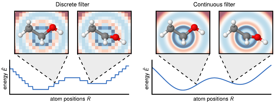
Figure from (Schütt et al. 2017): discrete vs continuous filter; continuous \(\to\) smooth energy surface.
The continuous-filter answer
\[ W(r) = \text{MLP}\!\left(\text{RBF}(r)\right) \in \mathbb{R}^F \]
- \(\text{RBF}(r)\) is a vector of Gaussian basis functions in \(r\).
- \(\text{MLP}\) is a small fully-connected network mapping the RBF expansion to \(F\) filter channels.
- \(W(r)\) is differentiable in \(r\) — gradients flow back to atomic positions for force prediction.
14. The SchNet update equation
Interaction block
For each atom \(i\) and each interaction layer \(t = 1, \ldots, T\):
\[ \mathbf{x}_i^{(t+1)} = \mathbf{x}_i^{(t)} + \sum_{j \in N(i)} \mathbf{x}_j^{(t)} \odot W^{(t)}\!\left(r_{ij}\right) \]
- \(\mathbf{x}_i^{(t)} \in \mathbb{R}^F\): atom \(i\)’s feature vector at layer \(t\).
- \(W^{(t)}(r_{ij}) \in \mathbb{R}^F\): continuous filter at this layer, evaluated at \(r_{ij}\).
- \(\odot\): element-wise (Hadamard) product.
- \(+\): residual connection.
Initialisation and readout
- \(\mathbf{x}_i^{(0)} = \text{Embed}(Z_i)\) — atom-type embedding.
- After \(T\) interactions, atom-wise MLP gives per-atom contributions \(E_i\).
- Total energy \(E = \sum_i E_i\) — extensive by construction.
- Forces \(\mathbf{F}_i = -\partial E / \partial \mathbf{r}_i\) via autograd.
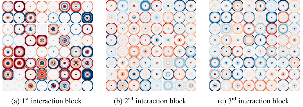
Learned radial filters \(W(r)\) in three SchNet interaction blocks (Schütt et al. 2017) — rotationally symmetric by construction.
15. Training on QM9
QM9 — the canonical molecular benchmark
- ~134k small organic molecules (up to 9 heavy atoms: C, N, O, F).
- DFT-computed properties: total energy, atomisation energy, HOMO/LUMO gap, dipole moment, polarisability, ZPVE, …
- Single-target regression on each property.
- Standard random or scaffold split.
SchNet’s QM9 result
- MAE on atomisation energy at chemical accuracy (\(\sim 1\) kcal/mol \(\approx 0.043\) eV).
- This level was previously reachable only via manually constructed feature pipelines.
- SchNet hit it end-to-end from atomic numbers and positions. That is the headline.
QM9 is the MNIST-like benchmark of early molecular machine learning: small, standardized, widely used, and focused on predicting quantum-mechanical properties from molecular structure.
16. What SchNet captures and what it misses
Captures
- Translation, rotation, permutation invariance by construction.
- Smooth, differentiable energy in \(\{\mathbf{r}_i\}\) \(\to\) usable forces via autograd.
- Local geometric environment via continuous distance filter.
- Extensive scaling via sum readout.
Misses
- Bond angles are not directly accessible (only via stacked distance filters that learn three-body indirectly).
- Forces are autograd-derived — correct, but not data-efficient.
- Long-range interactions need many interaction layers \(\to\) over-smoothing.
- Crystal-specific structure (lattice symmetry, unit-cell awareness) is not first-class.
17. Cutoff sensitivity and the smooth envelope
The cutoff problem
- Neighbour search uses a hard cutoff \(r_{\rm cut}\).
- An atom drifting just past \(r_{\rm cut}\) disappears from the neighbour list — discontinuously.
- Energy \(E\) jumps; forces \(\mathbf{F}_i = -\partial E / \partial \mathbf{r}_i\) blow up at the cutoff.
- This is a real MD failure mode.
The fix: a smooth envelope
- Multiply the filter by an envelope \(f_{\rm cut}(r)\) that goes smoothly to zero at \(r_{\rm cut}\): \[ W_{\rm smooth}(r) = W(r) \cdot f_{\rm cut}(r) \]
- Standard choices: cosine envelope, polynomial envelope.
- Now \(E\) and \(\mathbf{F}_i\) are continuous through the cutoff transition.
18. SchNet recap and bridge to CGCNN
One-slide SchNet summary
- Atoms \(\{Z_i, \mathbf{r}_i\}\) in.
- Atom embeddings \(\mathbf{x}_i^{(0)} = \text{Embed}(Z_i)\).
- \(T\) interaction layers with continuous-filter convolutions.
- Atom-wise MLP \(\to\) per-atom contributions.
- Sum \(\to\) total energy; autograd \(\to\) forces.
The SchNet \(\to\) CGCNN move
- SchNet treats each atom as identical except for its embedding.
- CGCNN adds explicit edge features and a gated update — the GNN-native version of SchNet.
- And CGCNN is designed from the start for crystals (PBC, periodic graphs).
- Same conceptual scaffold, more crystal-specific.
§D · CGCNN and message passing on crystal graphs
19. From molecules to crystals: CGCNN
The CGCNN setting (Xie and Grossman 2018)
- Input: a crystal — atoms in a unit cell with PBC.
- Graph: atoms as nodes, bonds (within a cutoff) as edges, including periodic-image bonds.
- Goal: predict a scalar property of the whole crystal.
- Foundational benchmark: Materials Project formation energy.
Why CGCNN matters
- First GNN designed natively for crystals — PBC are first-class.
- Achieved MAE of \(\sim 0.04\) eV/atom on formation energy on MP — close to DFT precision for many systems.
- Publicly released code + Materials Project hooks \(\to\) became the de facto benchmark for materials NN papers 2018–2022.
20. Edge attributes carry the geometry
Edge feature vector \(u_{ij}\)
- For each edge \((i, j)\), encode the interatomic distance \(r_{ij}\) via an RBF expansion (just like SchNet): \[ u_{ij} = [\exp(-\beta(r_{ij} - \mu_1)^2), \dots, \exp(-\beta(r_{ij} - \mu_K)^2)] \]
- \(K\) basis centres \(\mu_k\) spaced from \(0\) to \(r_{\rm cut}\).
- \(u_{ij} \in \mathbb{R}^K\).
Atom feature vector \(\mathbf{v}_i\)
- Initialised from the atomic number \(Z_i\) via a one-hot table (or learned embedding).
- Optionally enriched with chemistry priors (group, period, electronegativity, atomic radius) — see MG U7 slide 22.
- \(\mathbf{v}_i \in \mathbb{R}^F\).
The split. Chemistry enters via \(\mathbf{v}_i\). Geometry enters via \(u_{ij}\). The message-passing step on the next slide is what combines them.
21. The CGCNN gated convolution
The update
For each atom \(i\), layer \(t\):
\[ z_{ij} = [\mathbf{v}_i^{(t)} \,\|\, \mathbf{v}_j^{(t)} \,\|\, u_{ij}] \]
\[ \mathbf{v}_i^{(t+1)} = \mathbf{v}_i^{(t)} + \sum_{j \in N(i)} \sigma\!\left(W_z\, z_{ij} + b_z\right) \odot g\!\left(W_s\, z_{ij} + b_s\right) \]
- \(\sigma\): sigmoid (the gate).
- \(g\): nonlinearity (e.g. softplus).
- \(\odot\): Hadamard product.
- \(\|\): vector concatenation.
Reading the equation
- \(\sigma(W_z z_{ij} + b_z)\) is a gate in \([0, 1]^F\) — it decides how much of the message to pass.
- \(g(W_s z_{ij} + b_s)\) is the content of the message.
- The gate is per-channel, per-edge.
- Sum over neighbours \(\to\) permutation invariant.
- Residual \(+\) \(\to\) stable training across \(T\) layers.
22. Pooling: from atom features to a crystal property
Per-atom contributions
- After \(T\) message-passing layers, each atom has a feature \(\mathbf{v}_i^{(T)} \in \mathbb{R}^F\).
- An atom-wise MLP maps each \(\mathbf{v}_i^{(T)}\) to a per-atom contribution \(E_i \in \mathbb{R}\) (or to a per-atom feature for downstream pooling).
Crystal-level readout
- Sum for extensive properties (total energy, total magnetisation): \[ E = \sum_{i=1}^N E_i \]
- Mean for intensive properties (band gap, formation energy per atom, density of states): \[ \bar{E} = \frac{1}{N} \sum_i E_i \]
- Set2Set / attention for more flexible pooling (used in some MEGNet variants).
23. Connection back to MG U7
MG U7 sketched the schematic
- Crystal \(\to\) graph (PBC).
- Atom features \(\mathbf{v}_i\), edge features \(u_{ij}\).
- Message \(\to\) aggregate \(\to\) update.
- Repeat for \(T\) layers.
- Pool \(\to\) property.
CGCNN instantiates each piece
- Graph: PBC neighbour search, \(r_{\rm cut} = 8\) Å typical.
- \(\mathbf{v}_i\): 92-dim curated atom embedding.
- \(u_{ij}\): 41-dim Gaussian RBF of \(r_{ij}\).
- Message: \(\sigma(W_z z_{ij}) \odot g(W_s z_{ij})\).
- Pool: sum (energy) or mean (band gap).
The pedagogical reason for ordering MG U7 before MG U9. U7 builds the interface; U9 fills in the implementation. Once a student has the U7 schematic, every architecture in §D–§F is a different way of filling slots in that schematic.
24. Results: formation energy and beyond
Materials Project benchmarks (2018–2020)
- Formation energy: MAE \(\sim 0.04\) eV/atom on a random split; close to DFT precision for many systems.
- Band gap: MAE \(\sim 0.4\) eV — usable for screening, not for accurate prediction.
- Bulk / shear modulus: competitive with descriptor + RF baselines.
- Single trunk + multiple property heads \(\to\) multi-task variants.
Industrial use cases
- Battery cathode voltage screening (CGCNN, originally (Xie and Grossman 2018)).
- Catalyst formation-energy ranking on the Open Catalyst dataset (CGCNN as a baseline that newer architectures beat).
- High-throughput stability filter for ICSD- or MP-derived candidate lists.
25. CGCNN’s blind spots
What CGCNN does not see
- Bond angles (only pairwise distances).
- Three-body and higher correlations (no triplet edges).
- Long-range physics beyond \(T \cdot r_{\rm cut}\) (limited by depth and cutoff).
- Lattice-level symmetries beyond what is encoded in graph topology.
Why these blind spots matter
- Band-gap and elastic-modulus prediction strongly benefit from angles.
- Force prediction benefits from explicit three-body terms.
- Long-range Coulomb and dispersion physics need explicit handling.
- Each successor architecture in §E and §F addresses one or more of these.
§E · MEGNet, ALIGNN, M3GNet — the atom-bond-angle hierarchy
26. MEGNet: a set-of-graphs framing
The MEGNet generalisation (Chen et al. 2019)
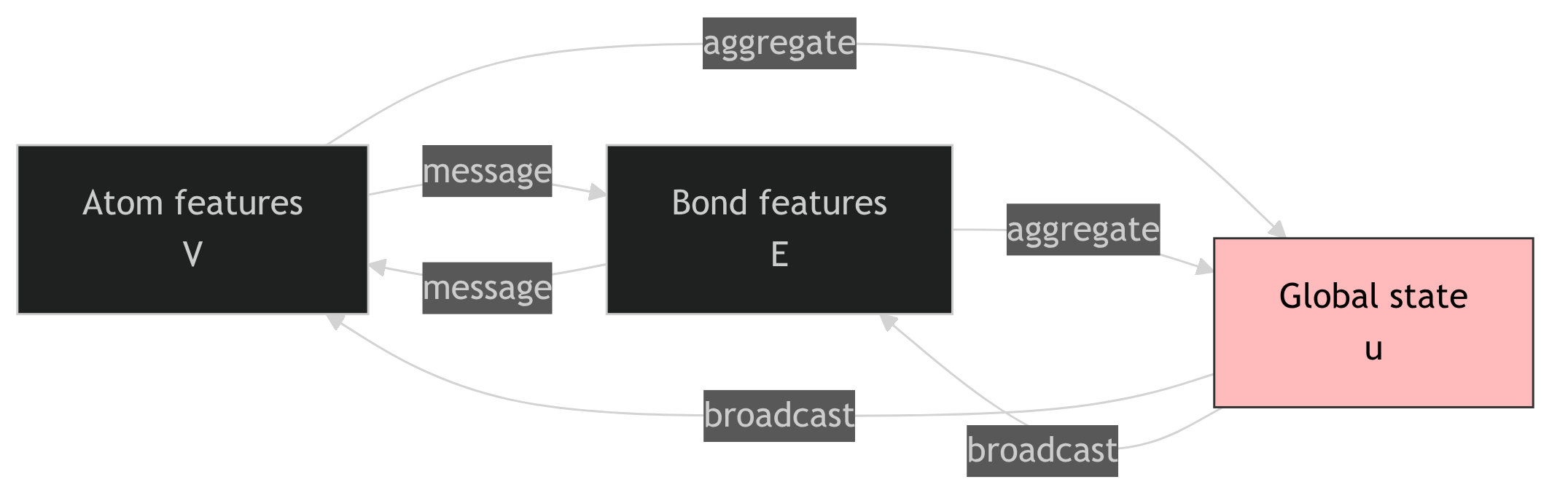
- Crystal as a tuple \((V, E, u)\):
- \(V = \{\mathbf{v}_i\}\): atom features.
- \(E = \{\mathbf{e}_{ij}\}\): bond features (full vectors, not just distances).
- \(u\): a global state vector (temperature, pressure, or learned token).
- Messages flow: atom \(\to\) bond \(\to\) atom \(\to\) global \(\to\) bond \(\to\) atom.
- Each round updates all three components.
27. Why the global state matters
Conditioning on external state
- \(u^{(0)}\) can carry: temperature \(T\), pressure \(P\), doping concentration, applied field.
- The same trunk then predicts \(E(T, P, \ldots)\), \(K(T, P, \ldots)\), etc.
- Multi-property heads share the trunk \(\to\) data efficiency for related properties.
Readout via the global state
- After \(T\) rounds, \(u^{(T)} \in \mathbb{R}^G\) is the crystal-level summary.
- A small MLP maps \(u^{(T)}\) to the predicted property.
- No separate pooling step — \(u\) does both jobs (state input and readout).
MEGNet on Materials Project (Chen et al. 2019). Multi-property heads (formation energy, band gap, bulk modulus, shear modulus) from a single trunk; competitive or better MAE than CGCNN on each.
28. ALIGNN: injecting bond angles via a line graph
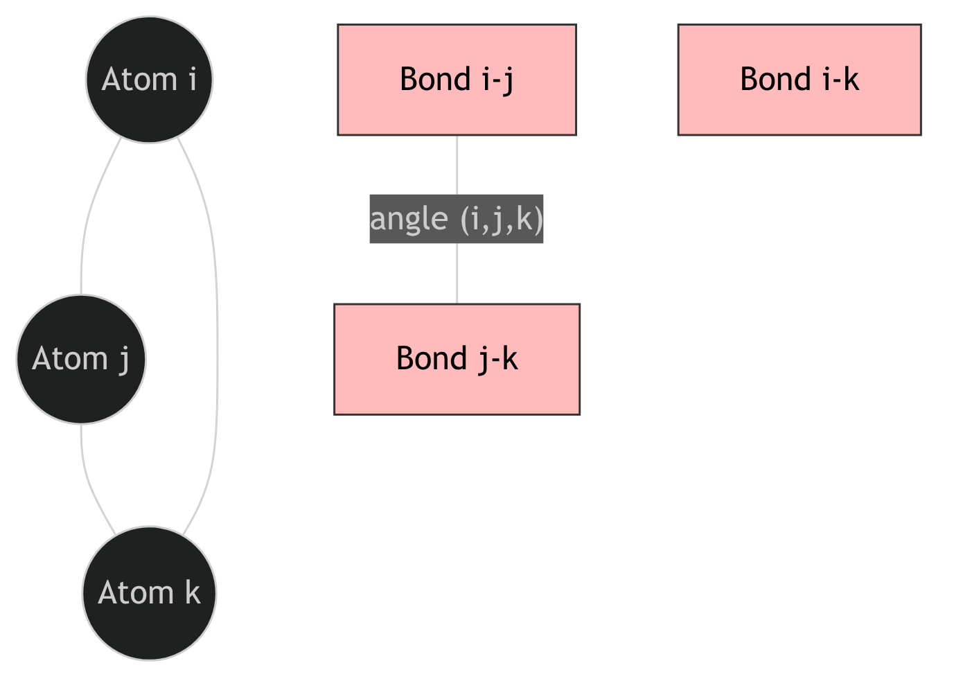
The ALIGNN trick (Choudhary and DeCost 2021)
- The original crystal graph \(G\) has nodes = atoms, edges = bonds.
- Construct the line graph \(L(G)\): nodes = bonds of \(G\), edges = pairs of bonds sharing an atom.
- A node of \(L(G)\) corresponds to a bond \((i, j)\); an edge of \(L(G)\) corresponds to a triplet \((i, j, k)\).
- Message passing on \(L(G)\) propagates angle information between bonds that share an atom.
- Alternate convolutions on \(G\) and \(L(G)\) to couple atom and angle channels.
29. The atom-bond-angle hierarchy
Increasing geometric resolution
| Architecture | Distances | Global state | Angles |
|---|---|---|---|
| SchNet | yes | — | — |
| CGCNN | yes | — | — |
| MEGNet | yes | yes | — |
| ALIGNN | yes | — | yes |
| M3GNet | yes | — | yes (3-body) |
- Each row adds at least one geometric channel.
- Each addition costs compute and parameters.
- Each addition pays off on the right property.
Which channel matters for which target
- Distances alone: good for formation energy, average bonding strength.
- + angles: crucial for band gap (depends on local symmetry), elastic moduli (depend on bond angles), defect stabilities.
- + global state: state-conditioned properties.
- + three-body terms: fine-grained MLIP forces, especially at finite T.
30. M3GNet: a foundation MLIP
M3GNet (Chen and Ong 2022)
- A universal machine-learning interatomic potential (MLIP).
- Trained across the periodic table on ~10⁵ MP relaxation trajectories (~10⁷ structures).
- Outputs energy + forces + stresses for arbitrary chemistry.
- Drop-in replacement for DFT in geometry optimisation and short MD.
Architectural extensions over MEGNet
- Explicit three-body interactions (atom–bond–bond triplets, like ALIGNN).
- Strict translation, rotation, permutation invariance for the energy.
- Forces and stresses obtained by autograd through positions and lattice.
- Smooth cutoffs to ensure physical force continuity.
31. The energy-force-stress contract
The three coupled outputs of an MLIP
- Energy: \(E(\{\mathbf{r}_i\}, \mathcal{L}) \in \mathbb{R}\) — invariant scalar.
- Forces: \(\mathbf{F}_i = -\dfrac{\partial E}{\partial \mathbf{r}_i} \in \mathbb{R}^3\) — equivariant vectors.
- Stress: \(\sigma = -\dfrac{1}{V}\dfrac{\partial E}{\partial \boldsymbol{\epsilon}} \in \mathbb{R}^{3 \times 3}\) — equivariant tensor.
Why the coupling is non-trivial
- All three must come from the same energy, by autograd.
- \(E\) must be smooth in \(\{\mathbf{r}_i\}\) and in lattice strains.
- Discontinuities in \(E\) \(\to\) blow-up in \(\mathbf{F}_i\) and \(\sigma\) \(\to\) MD crashes.
- Smooth-cutoff envelope, careful initialisation, force-stress-weighted loss.
The three-term loss. \[\mathcal{L} = \lambda_E \|E - E^{\rm DFT}\|^2 + \lambda_F \sum_i \|\mathbf{F}_i - \mathbf{F}_i^{\rm DFT}\|^2 + \lambda_\sigma \|\sigma - \sigma^{\rm DFT}\|^2\]
32. What each architecture is best at
| Architecture | Best for | Cost |
|---|---|---|
| CGCNN | Scalar property prediction; cheap workhorse baseline. | Low. |
| MEGNet | State-conditioned properties; multi-task heads from a shared trunk. | Low–medium. |
| ALIGNN | Properties depending on bond angles (band gap, elastic constants). | Medium. |
| M3GNet | Universal MLIP across the periodic table; energy + forces + stress. | High (deployment). |
| NequIP / MACE / Allegro (§F) | Small-data MLIP; force-accurate models from \(\sim 10^4\) structures. | High (per step). |
33. What they share
Shared scaffolding
- All operate on a (PBC-aware) crystal graph.
- All are translation-, rotation-, permutation-invariant for scalar outputs.
- All use distance-based filters or messages.
- All produce forces by autograd through energy.
- All scale linearly with the number of atoms (for fixed cutoff).
Shared limitation
- None carries explicit vector or tensor features in its hidden layers.
- All vector/tensor outputs (forces, stresses) come from autograd through invariant energy.
- This works, but is data-hungry — you need enough structures to imply the geometric covariance from energy variation alone.
- The §F architectures fix exactly this.
34. Materials-Project-scale results
Where the leaderboard sits in 2022–2023
- Formation energy: MAE \(\sim 0.02\) eV/atom (ALIGNN, M3GNet on MP-2021).
- Band gap: MAE \(\sim 0.25\) eV (ALIGNN).
- Elastic moduli: \(R^2 \sim 0.9\) on \(\sim 10^4\) training structures.
- Universal MLIP: M3GNet relaxes arbitrary MP entries to DFT minima zero-shot for most chemistries.
The ceiling shifted from model to data
- By 2022, MAE-on-random-split was not the bottleneck.
- The bottleneck became:
- DFT-functional inconsistency across MP versions.
- Polymorph aliasing in the dataset.
- Chemistry-grouped split degradation.
- Generalisation, not fitting.
- The MG U8 lesson became dominant.
§F · Equivariance done right
35. Why true equivariance matters
The autograd-from-invariants pathway
- Energy \(E\) is an invariant scalar.
- Forces \(\mathbf{F}_i = -\partial E / \partial \mathbf{r}_i\) — derived by autograd.
- Correct by construction.
- But: the network has no internal vector representation; it must infer directional information from the energy landscape variation.
The equivariant pathway
- Hidden features carry irrep labels: \(\ell = 0\) (scalars), \(\ell = 1\) (vectors), \(\ell = 2\) (rank-2 tensors), …
- Forces are native vector outputs from \(\ell = 1\) channels.
- Data efficiency improves by one to two orders of magnitude for force-rich tasks.
- Architectures: NequIP, Allegro, MACE.
The headline. For small-data MLIP regimes (~10⁴ structures, force labels), equivariant networks are the state of the art.
36. Irreducible-representation features
The irrep stack
- A representation of SO(3) decomposes into irreducible representations labelled by \(\ell = 0, 1, 2, \ldots\).
- \(\ell = 0\) — scalar (1-dimensional).
- \(\ell = 1\) — vector (3-dimensional).
- \(\ell = 2\) — symmetric traceless tensor (5-dimensional).
- An equivariant feature is a stack of irrep channels: \(\mathbf{x}_i = (x_i^{(0)}, x_i^{(1)}, x_i^{(2)}, \ldots)\).
Tensor products mix irreps
- Combining two irreps \(\ell_1 \otimes \ell_2\) produces a sum: \[\bigoplus_{|\ell_1 - \ell_2|}^{\ell_1 + \ell_2} \ell\]
- The Clebsch-Gordan coefficients control the mixing.
- The e3nn library implements all of this.
37. NequIP
NequIP (Batzner et al. 2022)
- The first widely-used E(3)-equivariant MLIP.
- Hidden features: scalars + vectors + tensors (irreps up to \(\ell \in \{1, 2\}\)).
- Message passing: Clebsch-Gordan tensor products of irrep features.
- Forces: native \(\ell = 1\) output (no autograd-only pathway).
The data-efficiency claim
- On force-rich catalyst and bulk-material datasets: \(\sim 1\)–2 orders of magnitude fewer training structures than non-equivariant baselines for the same force MAE.
- Now the standard small-data MLIP architecture.
- Codebase + tutorials at
mir-group/nequip.
38. Allegro and MACE
Allegro (Musaelian et al. 2023)
- Strictly local: each atom’s prediction depends only on its neighbourhood — no message passing across the graph.
- Trades expressiveness for parallelism.
- Scales to millions of atoms on a single GPU node.
- Right choice for large-cell MD where graph-wide message passing would exhaust memory.
MACE (Batatia et al. 2022)
- Replaces iterative message passing with higher-body-order tensor products in a single layer.
- 4-body and 5-body terms appear naturally.
- Comparable accuracy to NequIP at a fraction of the inference cost.
- Now the most popular small-data MLIP architecture.
39. The trade-off
When to go equivariant
- Small or medium dataset (\(\sim 10^3\)–\(10^5\) structures).
- Forces and stresses are central, not optional.
- Off-distribution chemistry expected at deployment.
- Implementation cost is acceptable (e3nn ecosystem).
When invariance + autograd is enough
- Large dataset (\(\sim 10^6\)+ structures).
- Energy-only or energy-dominant target.
- Inference latency must be minimal.
- Foundation-model pretraining available.
Rule of thumb. Crossover around \(\sim 10^5\) structures with strong force labels. Below: NequIP / MACE. Above: M3GNet / OMat24-style invariant + scale.
§G · Transformer-based variants and foundation models
40. Forward link to MFML W10
This section is a preview.
- MFML W10 will derive attention, multi-head attention, and transformer architectures.
- Today: how those primitives are applied to atomic systems.
- The goal: when MFML W10 lands, students recognise the materials use case.
What attention buys for crystals
- Long-range information without stacking many GNN layers.
- Global context: every atom can attend to every other atom in the cell.
- Pretraining + fine-tuning scales naturally: same primitives as NLP / vision foundation models.
- Foundation embeddings for materials become a tractable goal.
41. Matformer and Graphormer-style attention on crystals
Matformer (Yan et al. 2022)
- Transformer-style self-attention applied to crystal graphs.
- Each atom attends to all other atoms inside the cell.
- PBC-aware distance-based positional encoding (instead of NLP-style absolute position).
- Long-range interactions captured without stacking many message-passing layers.
Graphormer (Ying et al. 2021)
- Originally for molecular graphs; adapted to crystals in 2022–2023.
- Uses attention bias terms encoding shortest-path distances and bond features.
- Strong performance on both molecular and crystal benchmarks.
- Foundational for several 2024 materials transformers.
The architectural shift. Local message passing \(\to\) global attention. Receptive field = entire cell, in one layer. Compute cost scales as \(O(N^2)\) in atoms — manageable for typical unit cells, expensive for large supercells.
42. The OMat24 / GNoME / MatBERT generation
Foundation models reach materials (2023–2024)
- GNoME (Merchant et al. 2023): graph network trained on \(\sim 380\)k DFT structures, scaled iteratively via active learning to propose 2.2 million stable crystals.
- OMat24 (Barroso-Luque et al. 2024): the Open Materials 2024 dataset (~118 million DFT calculations) plus matching pretrained models for energy/force/stress.
- CHGNet, MatterSim, MACE-MP-0 (Batatia et al. 2024): foundation MLIPs covering the periodic table, distributed openly with Python APIs.
Multi-modal materials models
- MatBERT-style models: language-model pretraining on materials literature; produce text-side embeddings of materials concepts.
- Image + structure alignment: micrographs aligned with crystal structures via contrastive pretraining (analogue of CLIP for materials).
- Crystal + property + literature triples: the next generation of multi-modal foundation models for materials.
43. Pretraining vs fine-tuning for materials
The standard recipe (NLP-style)
- Pretrain on a broad corpus (~\(10^6\)–\(10^8\) DFT structures, energy + forces + stresses).
- Freeze or partially freeze the backbone.
- Fine-tune a small downstream head on the target dataset (~\(10^2\)–\(10^4\) labels).
- Deploy with task-specific calibration.
Why this works for materials
- Pretraining captures transferable physics: bonding, periodicity, local-environment statistics, force fields.
- Fine-tuning specialises to the idiosyncrasies of the target dataset (specific functional, specific chemistry, specific property).
- Data efficiency in fine-tuning rivals task-specific equivariant models.
The 2024–2026 default. New project? Start with a foundation-model checkpoint, fine-tune for a few hours. Train from scratch only if no relevant checkpoint exists.
44. The 2024–2026 state of the art
Where we are in 2026 (as of this lecture)
- Universal MLIPs at near-DFT force MAE on most chemistries.
- Foundation embeddings for materials available openly (OMat24, MACE-MP-0).
- Scaling laws apply: more data + more parameters = lower MAE.
- Multi-modal materials models (structure + text + property) emerging.
What is still missing
- Reliable extrapolation to genuinely novel chemistry / phases.
- Calibrated uncertainty for foundation-model predictions.
- Long-range physics beyond what attention captures (charge transfer, magnetism).
- Standardised benchmarks at MG U8 discipline level — the field is still catching up to grouped-split norms.
§H · Wrap-up
45. Decision tree: which architecture for which problem
By data regime
- Tens of structures: Magpie + RF / linear baseline; do not train a deep model.
- Hundreds–thousands: equivariant networks (NequIP, MACE, Allegro) or fine-tune a foundation model.
- Tens of thousands–millions: ALIGNN / M3GNet / Matformer; fine-tune a foundation model.
- Tens of millions+: train a foundation model from scratch (rarely justified at university scale).
By target type
- Composition-only properties: Magpie + MLP / RF.
- Scalar structure-dependent (formation energy, band gap): CGCNN / MEGNet / ALIGNN.
- Energy + forces (small data): NequIP / MACE / Allegro.
- Universal MLIP: M3GNet / CHGNet / MACE-MP-0 / OMat24.
- Long-range / global: Matformer / pretrained foundation model.
46. Small-data vs large-data regimes
Small-data (\(\sim 10^3\)–\(10^4\))
- Symmetry is the cheapest inductive bias.
- Equivariant networks dominate.
- Hand-crafted descriptors (MG U6) competitive.
- Fine-tuning a foundation model often beats both.
Large-data (\(\sim 10^5\)–\(10^8\))
- Symmetry still useful, often subsumed by data.
- Transformer-style attention competitive.
- Foundation-model pretraining dominates.
- The bottleneck shifts to data quality and split discipline (MG U8).
The crossover. Around \(\sim 10^5\) structures with strong force labels. Below: equivariance + handcrafted features. Above: pretrained foundation models + scale.
47. What we still inherit from MG U8
The MG U8 contract
- Grouped splits over chemistry / prototype.
- Residual analysis, not only scalar MAE.
- Skepticism of leaderboard scores.
- Effective sample size, not raw row count.
Applied to MG U9 architectures
- A Matformer that beats CGCNN on a random split but loses on a chemistry-grouped split is not the better model.
- A foundation model with \(10^8\) params and 0.02 eV/atom random-split MAE may have 0.20 eV/atom grouped-split MAE — and that 10× degradation matters.
- Architecture choice is a hypothesis to test, not a fashion to follow.
48. Bridge to Unit 10
Where we are
- §G ended with foundation models that output a transferable embedding for any atomic system.
- That embedding is a vector \(\mathbf{z} \in \mathbb{R}^d\) — the materials counterpart of an NLP word embedding.
- Today we trained it (via foundation-model pretraining); we did not study it.
Unit 10 picks up here
- Representation learning as the central object.
- The geometry of \(\mathbf{z}\)-space: similarity, clustering, manifold structure.
- Foundation embeddings for downstream tasks: similarity search, transfer learning, generative design.
- The bridge to the second half of the course.
The single sentence to leave with. Unit 9 produces the embedding; Unit 10 studies it.
Continue
49. References + reading map
Reading for next week
Recommended primary papers
- SchNet (Schütt et al. 2017, 2018).
- CGCNN (Xie and Grossman 2018).
- MEGNet (Chen et al. 2019).
- ALIGNN (Choudhary and DeCost 2021).
- M3GNet (Chen and Ong 2022).
- NequIP (Batzner et al. 2022).
- MACE (Batatia et al. 2022).
- Matformer (Yan et al. 2022).
- Open Materials 2024 (OMat24) (Barroso-Luque et al. 2024).
50. Exercise + Reading Assignment
Exercise (90 min, this afternoon)
- Build a CGCNN baseline on a curated Materials Project subset (formation energy or band gap). Use the MG U7 graph constructor; reuse MG U8’s grouped-split protocol.
- Compare against a Magpie + MLP baseline on the same grouped split. Report MAE, residuals by chemistry family, and one failure mode (e.g. cutoff sensitivity, polymorph aliasing).
- Bonus. Fine-tune a pretrained MACE-MP-0 checkpoint on the same task. Compare against your CGCNN.
Reading for next week
- Sandfeld et al. (2024), Ch 4.5 (must read).
- Neuer et al. (2024), Ch 4.5 (recommended).
- CGCNN (Xie and Grossman 2018) (recommended).
- MACE (Batatia et al. 2022) (optional).
Next week (Unit 10): representation learning — what to do with foundation-model embeddings. The supervised-architecture toolkit you learned today becomes the encoder for everything that follows.
Example Notebook
Week 10: Regression on Nanoindentation data — baseline NN models
![]()
© Philipp Pelz - Materials Genomics