Mathematical Foundations of AI & ML
Unit 5: Clustering and Autoencoders

Prof. Dr. Philipp Pelz

FAU Erlangen-Nürnberg

Where we are in the course

Behind us (Units 1-4):

• Risk minimization with labels: \((x_i, y_i)\) pairs.
• Linear models, generalized linear models, neural networks.
• Optimization (Unit 3) and architectures (Unit 4).

Today (Unit 5):

• The labels disappear: only \(\{x_i\}\) remains.
• Two complementary perspectives on finding structure without labels.
• Classical clustering (K-means, GMM) and neural autoencoders.

• The course pivot: from supervised to unsupervised.
• Why this matters: in materials work, labels are expensive (every label is a measurement).
• Two complementary perspectives meet here: classical (geometric/probabilistic) and neural (learned).

Note: backpropagation is self-study this term

• Unit 4 covered the architectures; how networks actually train (the chain rule, vanishing/exploding gradients) is in a self-study supplement.
• See 02_backprop_self_study.qmd in the Unit 4 folder, plus the two example notebooks 18.3_Backpropagation and 18.5_Python_Implementation.
• Today’s autoencoder section uses PyTorch autograd: loss.backward() handles the gradients.
• A short chain-rule warm-up is on the next exercise sheet

• Be explicit: backprop is essential; it is not skipped, only relocated.
• Modern practice: nobody implements backprop by hand at the use-site; autograd is the interface.
• The warm-up question makes sure they actually do the self-study.

The big leap

• All previous units assumed each datapoint comes with a target \(y_i\).
• In practice, most data has no labels: alloy compositions in a database, micrographs from a new sample, spectra from a new instrument.
• We can still ask: what structure is there? What groups together? What axes of variation matter?
• Today’s tools: clustering for discrete structure, autoencoders for continuous structure.

• Frame this as: the data is the only thing speaking; we listen.
• Materials motivations are real: most measurements are unlabeled until expensive characterization happens.

Learning outcomes

By the end of this unit, students can:

• Distinguish supervised vs unsupervised learning and recognize where each fits.
• Run K-means by hand on a small dataset and explain its convergence and failure modes.
• State the GMM likelihood and articulate why EM is needed when latent variables are present.
• Describe the autoencoder architecture and explain why a linear AE recovers PCA.
• Use an autoencoder for two practical tasks: data compression and anomaly detection.
• Anticipate how the latent space sets up Unit 9 (representation learning).

• Three tiers: classical clustering, autoencoder mechanics, applied use cases.
• Exam expectations: hand-trace K-means; identify clustering pathologies; reconstruct linear AE = PCA argument.

Roadmap of today’s 90 min

1. Unsupervised landscape (~10 min) — what counts as “structure”?
2. K-means (~15 min) — the workhorse.
3. Hierarchical clustering (~5 min) — when you don’t pick \(K\) in advance.
4. GMM + EM (~20 min) — probabilistic clustering.
5. Autoencoders (~25 min) — the neural counterpart.
6. Variants + applications (~10 min) — denoising, compression, anomaly detection.
7. Materials examples + bridge to Unit 6 (~5 min).

• Pace: each block is bounded; protect the AE block, it is the most novel for them.
• Skip K-medoids and hierarchical if running short — they are scaffolding.

The unsupervised landscape

• Clustering: assign each \(x_i\) to a discrete group.
• Dimensionality reduction: find low-dim coordinates that summarize \(x_i\).
• Density estimation: model \(p(x)\) directly.
• Generative modeling: sample new \(x \sim p(x)\). (Unit 11 will return here.)

Today: clustering (slides 6-32) and dimensionality reduction (slides 33-58). Density and generation come back in Units 8, 11, 12.

• Clustering and dim. reduction are the two foundational unsupervised tasks.
• Density estimation underlies generative modeling — coming later.
• Reinforce: these tasks are not mutually exclusive; an AE does dim. reduction and exposes clusters in the latent.

What counts as “structure”?

Compactness

Points within a group are close.

Separation

Groups are far from each other.

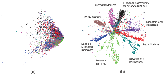
Plus: the structure must be interpretable — relate to something we care about (alloy family, defect type, processing regime). A “good” cluster on a materials dataset is one a metallurgist can explain.

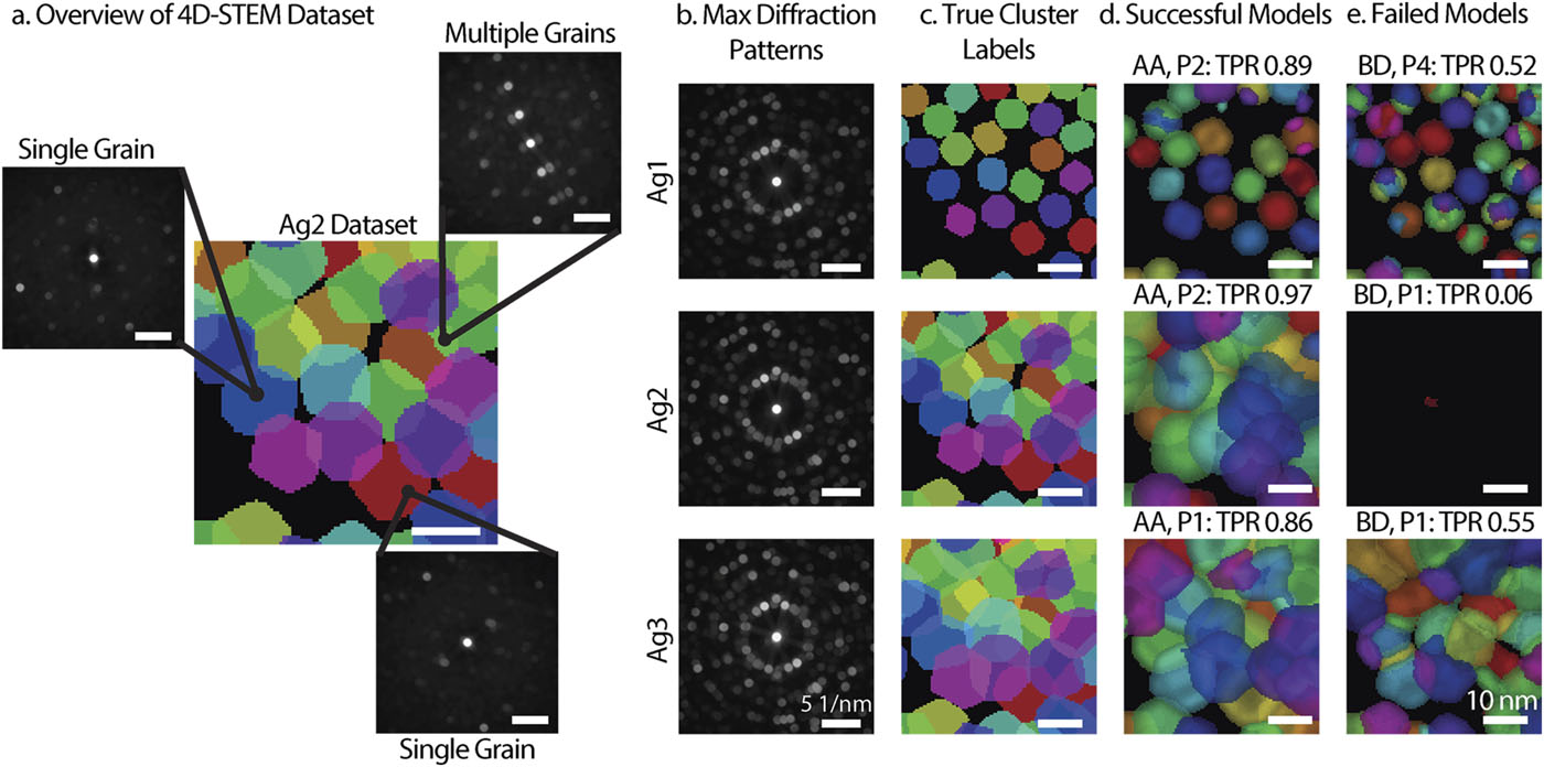
Overview of 4D-STEM with the visual representation of datasets and results. (a) Diagram of the 4D-STEM dataset. (b) Maximum diffraction patterns and (c) true cluster labels for the three simulated datasets, Ag1 (top), Ag2 (middle), and Ag3 (bottom). (d) Example of a successful model for each dataset. (e) Example of a failed model for each dataset. (Bruefach et al. 2023)

• Clustering quality is partly subjective: the math gives compactness and separation; meaning comes from the user.
• Materials example: unsupervised clustering that recovers known phase families is a sanity check; clusters that split a known family suggest a real discovery.

Why unsupervised matters in materials

• Most data starts unlabeled — a database of alloy compositions, a folder of micrographs, a stack of spectra.
• Labels often require expensive characterization (TEM, mechanical testing, EBSD).
• Unsupervised methods let us:
  • Explore before committing to a label scheme.
  • Compress (1000-channel spectrum → 10 latents).
  • Flag anomalies for expert attention before testing them all.

• Hammer the “labels are expensive” point: it is the everyday reason engineers reach for these methods.

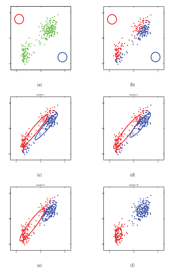
K-means: objective and Lloyd’s algorithm

Assign \(N\) points \(\{x_1, \ldots, x_N\} \subset \mathbb{R}^d\) to \(K\) groups \(C_1, \ldots, C_K\) by minimizing:

\[ J(C_1, \ldots, C_K, \mu_1, \ldots, \mu_K) = \sum_{k=1}^{K} \sum_{x_i \in C_k} \|x_i - \mu_k\|^2. \]

The objective: each point should be close to its assigned centroid. Each cluster is represented by a single point \(\mu_k\).

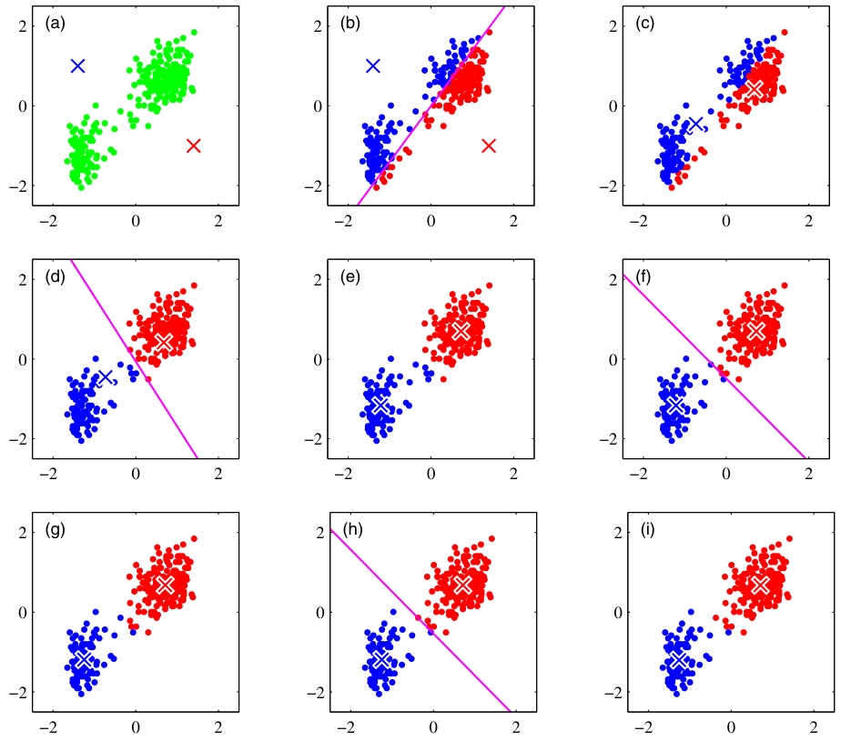
Lloyd’s algorithm

Alternate two steps until assignments stop changing:

1. Assign: for each \(i\), set \(C_k = \{x_i : k = \arg\min_j \|x_i - \mu_j\|^2\}\).
2. Update: for each \(k\), set \(\mu_k = \frac{1}{|C_k|} \sum_{x_i \in C_k} x_i\).

This is coordinate descent on \(J\): each step strictly decreases \(J\) unless we are already at a fixed point. Convergence in finitely many steps is guaranteed.

K-means iterations on the Old Faithful data (Bishop 2006, fig. 9.1). Each row shows one E-step (assign) and one M-step (update centroids). Converges in 3 M-steps.

• K is given (we will choose it later). Objective = within-cluster sum of squared distances; Euclidean distance must be meaningful for the features.
• Lloyd’s algorithm is what people mean by “K-means” in practice: coordinate descent, \(J\) monotone and nonnegative, finitely many steps; convergence is to a local optimum, not a global one.

Worked example: 6 points, \(K=2\)

Points: \((1,1), (1,2), (2,1)\), \((8,8), (9,8), (8,9)\).

Initial centroids: \(\mu_1 = (1,1)\), \(\mu_2 = (2,2)\).

viewof step = Inputs.range([0, 3], {step: 1, value: 0, label: "Algorithm Step"})

Step 0: Initialization.

Step 1: Assign to closest \(\mu\).

Step 2: Update \(\mu\) to cluster mean.

Step 3: Assign (No change).

The bad initialization still found the right clusters here — luck. With harder geometries, initialization matters a lot.

pts = [
  {id: 1, x: 1, y: 1}, {id: 2, x: 1, y: 2}, {id: 3, x: 2, y: 1},
  {id: 4, x: 8, y: 8}, {id: 5, x: 9, y: 8}, {id: 6, x: 8, y: 9}
];

// Precompute the steps
cents0 = [{x: 1, y: 1, c: "0"}, {x: 2, y: 2, c: "1"}];
asgn0 = pts.map(p => ({...p, c: "-1"})); 

asgn1 = pts.map(p => {
  let d0 = Math.hypot(p.x - cents0[0].x, p.y - cents0[0].y);
  let d1 = Math.hypot(p.x - cents0[1].x, p.y - cents0[1].y);
  return {...p, c: d0 < d1 ? "0" : "1"};
});
cents1 = cents0;

cents2 = [
  {x: (1+1+2)/3, y: (1+2+1)/3, c: "0"},
  {x: (8+9+8)/3, y: (8+8+9)/3, c: "1"}
];
asgn2 = asgn1;

asgn3 = pts.map(p => {
  let d0 = Math.hypot(p.x - cents2[0].x, p.y - cents2[0].y);
  let d1 = Math.hypot(p.x - cents2[1].x, p.y - cents2[1].y);
  return {...p, c: d0 < d1 ? "0" : "1"};
});
cents3 = cents2;

currentAsgn = [asgn0, asgn1, asgn2, asgn3][step];
currentCents = [cents0, cents1, cents2, cents3][step];

Plot.plot({
  width: 700,
  height: 700,
  grid: true,
  x: {domain: [0, 10]},
  y: {domain: [0, 10]},
  marks: [
    Plot.dot(currentAsgn, {x: "x", y: "y", fill: d => d.c === "-1" ? "gray" : (d.c === "0" ? "#1f77b4" : "#ff7f0e"), r: 10, stroke: "white", strokeWidth: 1}),
    Plot.dot(currentCents, {x: "x", y: "y", fill: d => d.c === "0" ? "#1f77b4" : "#ff7f0e", r: 16, symbol: "star", stroke: "black", strokeWidth: 1.5})
  ]
})

• Walk through this on the board.
• The point: K-means converges quickly when clusters are well-separated.
• Then transition to the failure modes.

K-means is sensitive to initialization

• Different initial centroids → different local optima.
• Standard fix: multiple random initializations, keep lowest \(J\).
• K-means++: smart initialization.
  • Pick first centroid randomly.
  • Pick next with probability \(\propto D(x)^2\) to nearest chosen centroid.
  • Provably bounds expected \(J\).

viewof initMethod = Inputs.radio(["Random", "K-means++"], {value: "Random", label: "Initialization"})
viewof rerunInit = Inputs.button("Run & Compare")

initData = {
  const n = 100;
  let data = [];
  const randn = () => Math.sqrt(-2.0 * Math.log(1 - Math.random())) * Math.cos(2.0 * Math.PI * Math.random());
  const centers = [{x: 0, y: 0}, {x: 4, y: 0}, {x: 4, y: 3}];
  for (let i = 0; i < n * 3; i++) {
    const c = centers[i % 3];
    data.push({x: c.x + randn()*0.8, y: c.y + randn()*0.8});
  }
  return data;
}

clusteredInit = {
  let trigger = rerunInit;
  let data = initData;
  let k = 3;
  let centroids = [];
  
  if (initMethod === "Random") {
    centroids = Array.from({length: k}, () => data[Math.floor(Math.random() * data.length)]);
  } else {
    // K-means++
    centroids.push(data[Math.floor(Math.random() * data.length)]);
    for (let i = 1; i < k; i++) {
      let dists = data.map(d => {
        let minDist = Infinity;
        for (let c of centroids) {
          let dist = Math.pow(d.x - c.x, 2) + Math.pow(d.y - c.y, 2);
          if (dist < minDist) minDist = dist;
        }
        return minDist;
      });
      let sumDist = dists.reduce((a, b) => a + b, 0);
      let r = Math.random() * sumDist;
      let cum = 0;
      for (let j = 0; j < data.length; j++) {
        cum += dists[j];
        if (cum >= r) {
          centroids.push(data[j]);
          break;
        }
      }
    }
  }
  
  let assignments = new Array(data.length).fill(0);
  for (let iter = 0; iter < 20; iter++) {
    let changed = false;
    for (let i = 0; i < data.length; i++) {
      let minDist = Infinity, minIdx = 0;
      for (let j = 0; j < k; j++) {
        let dist = Math.hypot(data[i].x - centroids[j].x, data[i].y - centroids[j].y);
        if (dist < minDist) { minDist = dist; minIdx = j; }
      }
      if (assignments[i] !== minIdx) { assignments[i] = minIdx; changed = true; }
    }
    if (!changed) break;
    let sums = Array.from({length: k}, () => ({x: 0, y: 0, count: 0}));
    for (let i = 0; i < data.length; i++) {
      sums[assignments[i]].x += data[i].x; sums[assignments[i]].y += data[i].y; sums[assignments[i]].count++;
    }
    for (let j = 0; j < k; j++) {
      if (sums[j].count > 0) {
        centroids[j].x = sums[j].x / sums[j].count; centroids[j].y = sums[j].y / sums[j].count;
      }
    }
  }
  return {data: data.map((d, i) => ({...d, cluster: String(assignments[i])})), centroids};
}

Plot.plot({
  width: 800,
  height: 800,
  grid: true,
  marks: [
    Plot.dot(clusteredInit.data, {x: "x", y: "y", fill: "cluster", stroke: "white", strokeWidth: 0.5, r: 5}),
    Plot.dot(clusteredInit.centroids, {x: "x", y: "y", fill: (d, i) => String(i), symbol: "star", r: 16, stroke: "black", strokeWidth: 1.5})
  ],
  color: {scheme: "category10"},
  axes: false
})

• K-means++ is the default in scikit-learn for a reason.
• For “\(D(x)^2\)”: for each point, compute distance to the nearest chosen centroid, square it, then sample proportionally. This makes far-away points much more likely, so seeds spread over different regions.
• For “provably bounds expected \(J\)”: in expectation over random seeding, the initial objective is within a logarithmic factor of the optimal \(K\)-means objective (about \(O(\log K)\) times optimum), so this is a true theoretical guarantee.
• Practical advice: always use K-means++ and a few restarts.

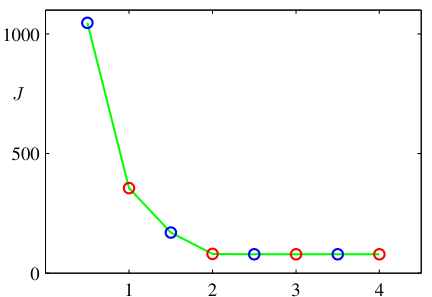
Choosing \(K\): the elbow method

• Run K-means for \(K = 1, 2, 3, \ldots, K_{\max}\).
• Plot \(J(K)\) vs \(K\).
• Look for the elbow: the point where \(J\) stops dropping fast.
• Heuristic, not principled, but widely used.

\(J(K)\) always decreases with \(K\) — at \(K = N\), every point is its own cluster and \(J = 0\).

The elbow signals diminishing returns from extra clusters.

Cost function \(J\) after each E-step (blue) and M-step (red) for the Old Faithful example. Converged after 3 M-steps. (Bishop 2006, fig. 9.2)

• The elbow is sometimes obvious (sharp bend), often not (smooth curve).
• Combine with the silhouette score for a second opinion.

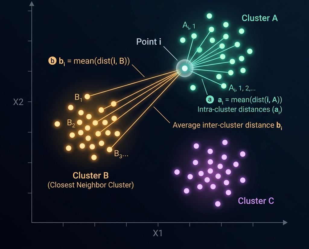
Choosing \(K\): the silhouette score

For each point \(x_i\), define:

\[ s(x_i) = \frac{b(x_i) - a(x_i)}{\max(a(x_i), b(x_i))}, \]

where \(a(x_i)\) is the average distance to other points in \(x_i\)’s cluster, and \(b(x_i)\) is the average distance to points in the nearest other cluster.

• \(s(x_i) \approx 1\): well-clustered. \(s(x_i) \approx 0\): on a boundary. \(s(x_i) < 0\): probably misclustered.
• Pick the \(K\) that maximizes the mean silhouette.

Visual interpretation of the silhouette score components: \(a(x_i)\) measures intra-cluster cohesion, while \(b(x_i)\) measures inter-cluster separation.

• Silhouette gives a per-point quality score and an aggregate.
• Use elbow + silhouette together; if they agree, more confidence.
• Don’t oversell either: clustering quality is ill-defined.

K-means: the spherical assumption

• K-means uses Euclidean distance to a single centroid.
• Implicitly assumes clusters are spherical and equal-sized.
• Fails when:
  • Clusters are elongated (Anisotropic).
  • Geometry is non-convex (Moons, Rings).

These failure cases motivate GMM (slides 24+).

viewof datasetShape = Inputs.radio(
  ["Blobs", "Moons", "Concentric Rings", "Anisotropic"], 
  {label: "Dataset Shape", value: "Moons"}
)
viewof rerun = Inputs.button("Re-run K-means")

points = {
  let trigger = rerun; // depend on button
  const n = 400;
  let data = [];
  const randn = () => Math.sqrt(-2.0 * Math.log(1 - Math.random())) * Math.cos(2.0 * Math.PI * Math.random());
  
  if (datasetShape === "Blobs") {
    const centers = [{x: 0, y: 0}, {x: 5, y: 5}, {x: 0, y: 5}];
    for (let i = 0; i < n; i++) {
      const c = centers[i % 3];
      data.push({x: c.x + randn(), y: c.y + randn()});
    }
  } else if (datasetShape === "Moons") {
    for (let i = 0; i < n/2; i++) {
      const t = Math.PI * Math.random();
      data.push({x: Math.cos(t) + randn()*0.1, y: Math.sin(t) + randn()*0.1});
      data.push({x: 1 - Math.cos(t) + randn()*0.1, y: 1 - Math.sin(t) - 0.5 + randn()*0.1});
    }
  } else if (datasetShape === "Concentric Rings") {
    for (let i = 0; i < n/2; i++) {
      const t = 2 * Math.PI * Math.random();
      data.push({x: 0.5 * Math.cos(t) + randn()*0.05, y: 0.5 * Math.sin(t) + randn()*0.05});
      data.push({x: 1.5 * Math.cos(t) + randn()*0.05, y: 1.5 * Math.sin(t) + randn()*0.05});
    }
  } else if (datasetShape === "Anisotropic") {
    for (let i = 0; i < n; i++) {
      const c = (i % 3);
      let rx = randn(); let ry = randn();
      let rotX = rx * 0.866 - ry * 0.5;
      let rotY = rx * 0.5 + ry * 0.866;
      if (c === 0) data.push({x: rotX*3 - 4, y: rotY*0.5 - 4});
      else if (c === 1) data.push({x: rotX*3, y: rotY*0.5});
      else data.push({x: rotX*3 + 4, y: rotY*0.5 + 4});
    }
  }
  return data;
}

// K-means
clusteredData = {
  let data = points;
  let k = datasetShape === "Concentric Rings" ? 2 : (datasetShape === "Moons" ? 2 : 3);
  let centroids = Array.from({length: k}, () => data[Math.floor(Math.random() * data.length)]);
  let assignments = new Array(data.length).fill(0);
  
  for (let iter = 0; iter < 20; iter++) {
    let changed = false;
    for (let i = 0; i < data.length; i++) {
      let minDist = Infinity, minIdx = 0;
      for (let j = 0; j < k; j++) {
        let dist = Math.hypot(data[i].x - centroids[j].x, data[i].y - centroids[j].y);
        if (dist < minDist) { minDist = dist; minIdx = j; }
      }
      if (assignments[i] !== minIdx) { assignments[i] = minIdx; changed = true; }
    }
    if (!changed) break;
    let sums = Array.from({length: k}, () => ({x: 0, y: 0, count: 0}));
    for (let i = 0; i < data.length; i++) {
      sums[assignments[i]].x += data[i].x; sums[assignments[i]].y += data[i].y; sums[assignments[i]].count++;
    }
    for (let j = 0; j < k; j++) {
      if (sums[j].count > 0) {
        centroids[j].x = sums[j].x / sums[j].count; centroids[j].y = sums[j].y / sums[j].count;
      }
    }
  }
  return data.map((d, i) => ({...d, cluster: String(assignments[i])}));
}

Plot.plot({
  width: 600,
  height: 450,
  grid: true,
  marks: [
    Plot.dot(clusteredData, {x: "x", y: "y", fill: "cluster", stroke: "white", strokeWidth: 0.5, r: 5})
  ],
  color: {scheme: "category10"},
  axes: false
})

• This is the most important limitation to internalize: spherical clusters only.
• The classical “two moons” dataset breaks K-means in a way that motivates kernel methods or DBSCAN — but here we move to GMM.

K-medoids: a robust variant

• K-means uses the mean as a centroid → sensitive to outliers.
• K-medoids restricts the centroid to be an actual data point (the medoid).
• Update step: in each cluster, pick the point that minimizes the sum of distances to others.
• Slower (no closed-form update) but robust.

Useful when: outliers contaminate the data, or distances are non-Euclidean (e.g., edit distance for SMILES strings).

The K-means centroid (orange cross) is pulled away from the main cluster by a single outlier, whereas the K-medoid (blue circle) remains safely anchored to a real data point in the dense region.

• K-medoids is what you reach for when K-means breaks due to outliers.
• Mention as a tool; we won’t go deeper.

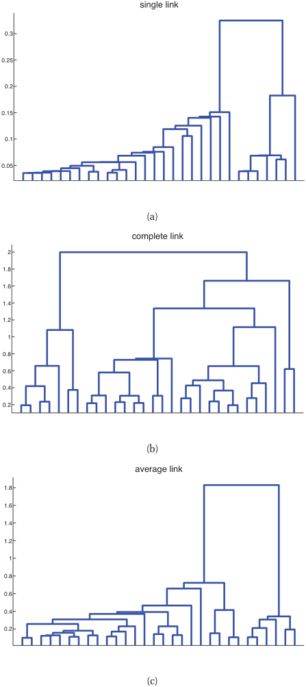
Hierarchical clustering: no \(K\) in advance

• Agglomerative: start with each point as its own cluster; repeatedly merge the closest pair.
• Divisive: start with one big cluster; recursively split.
• Linkage criteria for “closest”:
  • Single: nearest pair across clusters (chains).
  • Complete: farthest pair (compact).
  • Average: mean pair distance.
  • Ward: minimize variance increase (popular default).

Visual comparison of linkage criteria between two clusters. The top line shows Single Linkage (closest points), the middle line shows Average Linkage, and the bottom line shows Complete Linkage (furthest points).

• Useful when K is not known a priori, or when the hierarchy itself is informative (e.g., taxonomy of alloys).
• Ward linkage gives K-means-like geometric clusters and is generally the most robust default.
• Implementation in Python (scikit-learn / SciPy):
  • Agglomerative is fully supported via sklearn.cluster.AgglomerativeClustering, which uses Ward linkage by default.
  • Scikit-learn does not implement pure Divisive clustering (although BisectingKMeans exists as a top-down K-means variant).
  • To actually visualize the hierarchy (dendrograms, which are on the next slide), students will need to use scipy.cluster.hierarchy because sklearn is designed to just return flat cluster labels.

Dendrograms

• The merge sequence is a tree: leaves are points, internal nodes are merges, height = merge distance.
• Cut the dendrogram at any height to obtain a clustering.
• Materials use case: dendrograms over compositions reveal natural alloy families and the heights tell you how distinct each family is.
• Linkage choice matters: single, complete, average, or Ward produce qualitatively different trees.

Effect of linkage on the dendrogram for yeast gene-expression data: (a) single link — chaining artifacts; (b) complete link — compact clusters; (c) average link — a compromise. (Murphy 2012, fig. 25.15)

• Dendrogram cut height is the analog of choosing K.
• Hierarchical clustering scales as O(N^2 log N) — fine for thousands of points, slow for millions.

From hard to soft assignments

• K-means gives a hard assignment: each point belongs to exactly one cluster.
• Reality: a point near a boundary could plausibly belong to either neighbor.
• A soft assignment gives a probability over clusters: \(\gamma_{ik} = P(\text{cluster } k \mid x_i)\).
• Soft assignments come naturally from a probabilistic model: the Gaussian Mixture Model.

Same 500 points from a 3-Gaussian mixture: (a) complete data with hard labels, (b) unlabeled (incomplete data), (c) soft coloring by responsibilities \(\gamma_{ik}\) — purple = uncertain. (Bishop 2006, fig. 9.5)

• The shift to GMM is conceptual: model the data, not just partition it.
• Probabilities give us uncertainty over assignments — useful for downstream decisions.

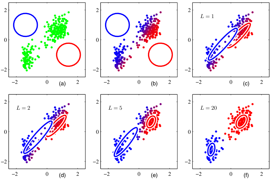
Gaussian Mixture Model (GMM)

A weighted sum of \(K\) Gaussian densities:

\[ p(x) = \sum_{k=1}^{K} \pi_k \mathcal{N}(x; \mu_k, \Sigma_k), \qquad \pi_k \geq 0, \quad \sum_k \pi_k = 1. \]

• \(\pi_k\): mixture weight (prior probability of cluster \(k\)).
• \(\mu_k\): cluster center; \(\Sigma_k\): cluster shape (covariance).
• Each \(\mathcal{N}(x; \mu_k, \Sigma_k)\) is a multivariate Gaussian — Unit 7 will derive these formally.

A mixture of 3 Gaussians in 2D: (a) contours of each component; (b) the combined density surface. Each component can have its own shape and orientation. (Murphy 2012, fig. 11.3)

• The GMM is what you get when each point is generated from one of K Gaussians, but you don’t know which.
• Generality vs K-means: ellipsoidal clusters of any orientation and any relative size.

The latent variable view

Introduce \(z_i \in \{1, \ldots, K\}\) — the (unobserved) cluster index for \(x_i\).

\[ p(x_i, z_i = k) = \pi_k \mathcal{N}(x_i; \mu_k, \Sigma_k), \qquad p(x_i) = \sum_k p(x_i, z_i = k). \]

• We observe \(x_i\) and don’t observe \(z_i\).
• Maximizing \(\log p(x_i; \theta)\) directly is hard because it contains a sum inside the log.
• The trick: alternate between guessing \(z_i\) and updating \(\theta\). This is EM.

• The latent variable formulation is the gateway to EM.
• “Sum inside log” makes the gradient ugly — EM sidesteps this.

EM algorithm: E-step

For each point \(i\) and cluster \(k\), compute the responsibility:

\[ \gamma_{ik} = P(z_i = k \mid x_i, \theta) = \frac{\pi_k \mathcal{N}(x_i; \mu_k, \Sigma_k)}{\sum_{j} \pi_j \mathcal{N}(x_i; \mu_j, \Sigma_j)}. \]

This is the soft assignment: how strongly does the model believe point \(i\) belongs to cluster \(k\), given the current parameters?

EM algorithm: M-step

Update parameters using the responsibilities:

\[ \mu_k = \frac{\sum_i \gamma_{ik} x_i}{\sum_i \gamma_{ik}}, \qquad \Sigma_k = \frac{\sum_i \gamma_{ik} (x_i - \mu_k)(x_i - \mu_k)^T}{\sum_i \gamma_{ik}}, \qquad \pi_k = \frac{1}{N}\sum_i \gamma_{ik}. \]

Each update is a weighted average — points contribute to a cluster in proportion to their responsibility.

EM for GMM on Old Faithful: (a) initial random parameters; (b) responsibilities after 1st E-step (purple = uncertain); (c)–(f) convergence over 16 iterations. (Murphy 2012, fig. 11.11)

• E-step uses Bayes’ rule (Unit 7 will treat this formally).

• Compare to K-means: there, \(\gamma_{ik}\) is 0 or 1 (hard).

• M-step is intuitive: weighted least-squares update for the means, weighted covariance, weighted prior.

• The closed-form M-step is what makes EM tractable for GMMs.

EM as alternating optimization

1. Initialize \(\{\pi_k, \mu_k, \Sigma_k\}\) (e.g., from K-means output).
2. E-step: compute all \(\gamma_{ik}\) given current parameters.
3. M-step: update parameters given current \(\gamma_{ik}\).
4. Repeat until log-likelihood converges.

Property: each EM iteration is guaranteed not to decrease the data log-likelihood \(\sum_i \log p(x_i; \theta)\). (Proof: EM optimizes a lower bound on the log-likelihood — Bishop Ch. 9 has the full derivation.)

EM for a 2-component GMM on the Old Faithful data. (a) initialization; (b)–(f) E/M steps shown with soft color-coded responsibilities. Ellipses show the 1-\(\sigma\) contours of each Gaussian. (Bishop 2006, fig. 9.8)

• EM is structurally identical to coordinate ascent: alternate over (z, theta).
• Like K-means, EM converges to a local optimum; initialization matters.
• Common practice: initialize EM with the output of K-means.

K-means vs GMM

	K-means	GMM
Assignment	hard	soft
Cluster shape	spherical	ellipsoidal (full \(\Sigma\))
Cluster size	implicit	learned via \(\Sigma\)
Output	partition	density
Cost	\(O(NKd)\) per iter	\(O(NKd^2)\) per iter

Rule of thumb: K-means for fast, geometric, well-separated clusters. GMM when clusters overlap, vary in shape, or you need probabilities downstream.

• A GMM with shared identity covariance and equal mixture weights, in the limit of small variance, recovers K-means. (Mention as trivia; do not derive.)

Choosing \(K\) for GMM: BIC

The Bayesian Information Criterion penalizes complexity:

\[ \text{BIC}(K) = -2 \log p(\mathcal{D}; \hat\theta_K) + p_K \log N, \]

where \(p_K\) is the number of free parameters in a \(K\)-component GMM.

• Fit GMMs for \(K = 1, 2, \ldots\), pick the \(K\) minimizing BIC.
• BIC works because GMM has a likelihood. K-means does not — that’s why we used elbow/silhouette there.

• BIC is the principled answer to “how many clusters?” when you have a likelihood.
• Connect to Unit 7: this is essentially Bayesian model comparison via marginal likelihood approximation.
• Derivation of \(p_K\) (free parameters) to show on board: For a \(K\)-component GMM in \(d\) dimensions:
  • Mixture weights (\(\pi_k\)): \(K - 1\) (because they sum to 1).
  • Means (\(\mu_k\)): \(K \times d\).
  • Covariance matrices (\(\Sigma_k\)):
    • Full: \(K \times \frac{d(d+1)}{2}\) (symmetric matrix)
    • Diagonal: \(K \times d\)
    • Spherical: \(K \times 1\)
  • Total (full covariance): \(p_K = (K - 1) + Kd + K\frac{d(d+1)}{2}\).
• Mention this briefly: it explains why BIC heavily penalizes full-covariance GMMs in high dimensions compared to K-means!

Bridge: from centroids to learned representations

• K-means represents each cluster by a single point \(\mu_k\).
• GMM represents each cluster by a distribution \(\mathcal{N}(\mu_k, \Sigma_k)\).
• Both compress the data into a small number of “summary” objects.
• What if we want continuous structure — a smooth low-dimensional surface that describes the data?

That is what an autoencoder learns. The encoder maps \(x\) to a low-dim latent code \(z\); the decoder reconstructs \(x\) from \(z\).

• The pivot: clustering finds discrete structure; autoencoders find continuous structure.
• This is also the bridge to Unit 9 (representation learning) and Unit 11 (generative models).

The manifold hypothesis

• High-dimensional data is rarely “filled in” — a 1024-channel spectrum lives in \(\mathbb{R}^{1024}\), but real spectra concentrate on a much lower-dimensional surface (manifold).
• The manifold’s intrinsic dimension is governed by physics (number of phases, processing parameters).
• A linear method (PCA) finds a flat low-dim subspace.
• A nonlinear method (autoencoder) can curve to follow the manifold.

• Manifold hypothesis: real data lives near a low-dim surface in a high-dim ambient space.
• Examples: alloy compositions (constrained by phase rules); micrographs (constrained by physics of imaging).

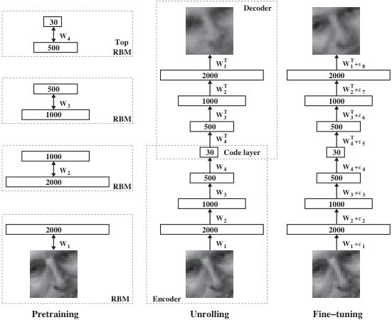
The autoencoder architecture

        encoder              decoder
   x  ──────►  z (bottleneck)  ──────►  x̂
 R^d           R^k (k ≪ d)              R^d

• Encoder \(f_\phi: \mathbb{R}^d \to \mathbb{R}^k\): compresses input to a code \(z\).
• Bottleneck \(z \in \mathbb{R}^k\): forced low-dimensional representation.
• Decoder \(g_\theta: \mathbb{R}^k \to \mathbb{R}^d\): reconstructs input from code.
• Loss: reconstruction error, typically MSE.

A deep autoencoder: (a) greedily pre-train RBM layers; (b) unroll into encoder/decoder by tying weights; (c) fine-tune end-to-end with backprop. The bottleneck (middle layer) is the latent code \(z\). (Murphy 2012, fig. 28.3)

• Hourglass topology: wide → narrow → wide.
• Both encoder and decoder are neural networks; in the simplest case, they are MLPs.

The reconstruction objective

\[ \mathcal{L}(\theta, \phi) = \frac{1}{N}\sum_{i=1}^{N} \|x_i - g_\theta(f_\phi(x_i))\|^2. \]

• No labels — only the inputs themselves serve as targets.
• Minimizing \(\mathcal{L}\) forces the bottleneck \(z\) to retain enough information to reconstruct \(x\).
• Without the bottleneck, the network could just learn the identity. The bottleneck creates a useful constraint.

• Self-supervised: the supervisory signal comes from the data itself.
• The bottleneck is the soul of the autoencoder.

Linear autoencoder = PCA

Take the simplest possible AE:

\[ f_\phi(x) = W_e x, \qquad g_\theta(z) = W_d z, \qquad W_e \in \mathbb{R}^{k \times d}, \quad W_d \in \mathbb{R}^{d \times k}. \]

Theorem. With MSE loss, the optimal \((W_e, W_d)\) satisfy \(W_d W_e = U_k U_k^T\), where \(U_k\) contains the top-\(k\) left singular vectors of the centered data — i.e., the PCA subspace.

A linear autoencoder is just PCA in disguise.

• This is a deep result: it tells us autoencoders generalize PCA.
• Derivation outline (for the board or if asked):
  • The objective is \(\min_{W_d, W_e} \sum_i \| x_i - W_d W_e x_i \|^2\).
  • Let \(P = W_d W_e\). Since \(W_e\) is \(k \times d\) and \(W_d\) is \(d \times k\), \(P\) is a matrix of rank at most \(k\).
  • By the Eckart-Young-Mirsky theorem (from linear algebra), the rank-\(k\) matrix \(P\) that minimizes the squared reconstruction error is the orthogonal projection onto the top-\(k\) principal subspace.
  • Therefore, \(P = U_k U_k^T\), where \(U_k\) holds the top \(k\) principal components (eigenvectors of the covariance matrix).
  • Thus, \(W_d W_e = U_k U_k^T\). A natural solution is \(W_d = U_k\) and \(W_e = U_k^T\).
• Crucial point: The solution is unique only up to a linear transformation in the latent space. For any invertible \(k \times k\) matrix \(M\), \(W_d' = W_d M\) and \(W_e' = M^{-1} W_e\) yields the same reconstruction \(P\).
• So the AE finds the same subspace as PCA, but its specific latent variables \(z\) might just be a rotated or scaled version of the true PCA scores.

Why nonlinearity matters

• Linear AEs find the best flat subspace.
• Real data manifolds are usually curved: alloy compositions on a phase diagram, micrographs under varying lighting.
• Adding a nonlinearity (ReLU, tanh) and a hidden layer to encoder and decoder lets the AE bend the latent space.
• Result: a nonlinear AE can capture variance that PCA leaves on the table.

This is the same lesson as Unit 4: nonlinearity is what lets neural networks go beyond linear models.

• The contrast with PCA is the cleanest “why neural” argument we have for unsupervised work.
• For students: PCA is a special case; the AE is the general tool.

Choosing the bottleneck dimension \(k\)

• Too small: the AE underfits — reconstruction is bad even on training data.
• Too large: the AE overfits — it just learns the identity through a wide pipe.
• Procedure: sweep \(k\), plot validation reconstruction error vs \(k\), look for the elbow.
• Sanity check: compare to PCA at the same \(k\). Nonlinear AE should do at least as well.

• Bottleneck size is the most important hyperparameter for an AE.
• Always compare against PCA at the same dim — a good baseline.

Convolutional autoencoders

For spatial data (images, fields), use convolution:

• Encoder: stack of strided conv → pool blocks (downsample).
• Decoder: stack of transposed conv (or upsample + conv) blocks.
• The bottleneck is now a small feature map.

• Same architectural reasoning as Unit 4: locality + weight sharing.
• Materials uses: micrograph compression, simulation field compression.

• Conv AEs reuse all of Unit 4’s vocabulary.
• Transposed convolution is the natural inverse to strided convolution; mention “checkerboard artifacts” briefly.

Training: autograd handles it

• An AE is a standard neural network with a peculiar loss.

• PyTorch:

  loss = ((x - decoder(encoder(x)))**2).mean()
  loss.backward()
  optimizer.step()

• All the backprop machinery (chain rule, gradient flow, Xavier/He init) from the self-study supplement applies here directly.

• This is where the self-study payoff matters: students should know what backward() does, even if they never write it.
• Optimizer choice: Adam by default, more in Unit 6.

Denoising autoencoder

Train the AE with corrupted inputs:

\[ \mathcal{L} = \frac{1}{N}\sum_i \|x_i - g_\theta(f_\phi(\tilde x_i))\|^2, \qquad \tilde x_i = x_i + \epsilon_i. \]

• The AE must denoise — recover the clean \(x_i\) from a noisy \(\tilde x_i\).
• Forces the latent code to capture robust features, not noise.
• Practical hyperparameter: noise level. Too low → trivial; too high → unrecoverable.

• Denoising AE is one of the most common training tricks.
• It also connects to score-based generative models — Unit 11 will revisit.

Sparse autoencoders (briefly)

• Add a penalty that encourages most latent activations to be near zero.
• Forces the AE to use few latent units per input — interpretable, disentangled features.
• Loss: \(\mathcal{L}_{\text{recon}} + \lambda \|z\|_1\) (Lasso-like) or KL penalty against a Bernoulli prior.

• Mention briefly; full disentanglement is its own research area.
• In materials, sparsity helps interpretability: which 3-of-128 latents represent “this is martensite”?

Application 1 — anomaly detection

• Train the AE only on normal data.
• At test time, compute reconstruction error per sample.
• Anomalies (defects, instrument failures, novel phases) reconstruct poorly — they’re outside the manifold the AE learned.
• Threshold: choose at, say, the 99th percentile of training reconstruction error.

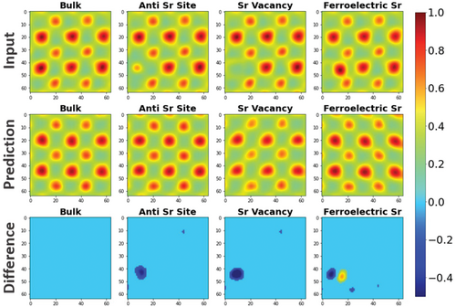
Short Story: Crystal Defect Detection Prifti et al. (2023) used a Convolutional Variational Autoencoder (CVAE) on Scanning Transmission Electron Microscopy (STEM) images. Trained purely on perfect crystal lattices, the CVAE flags point defects (e.g., vacancies or anti-sites) simply because it fails to reconstruct them. It identifies anomalies without ever seeing a defect during training!

• Anomaly detection without labeled defects is one of the most valuable AE applications in industry.
• The Prifti et al. (2023) paper in Small perfectly illustrates this in materials science.
• Choosing the threshold is a per-application calibration question.

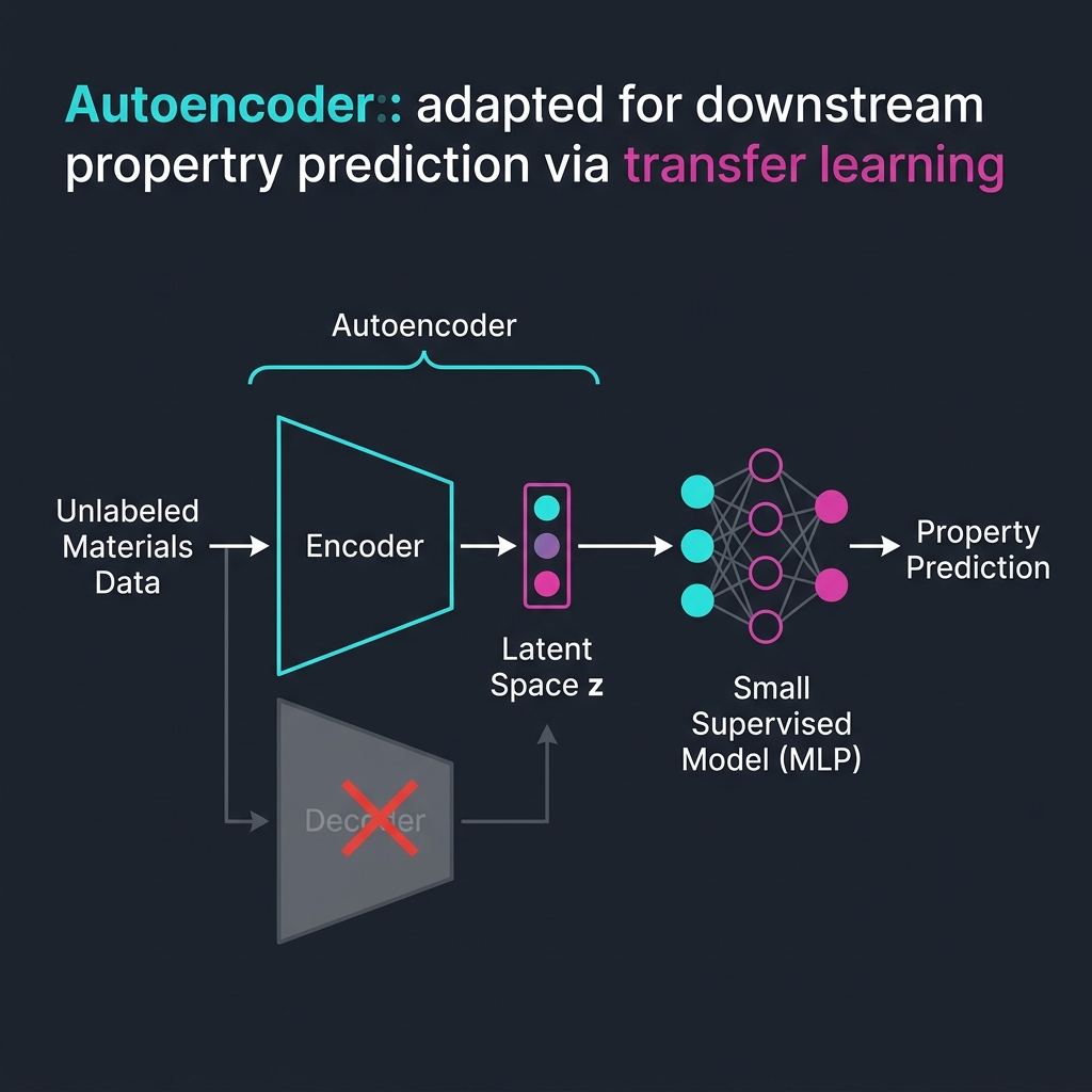
Application 2 — features for downstream tasks

• Train an AE on a large unlabeled corpus.
• Discard the decoder; use the encoder \(z = f_\phi(x)\) as a feature extractor.
• Train a small supervised model (linear regression, MLP) on \(z\) instead of \(x\).
• Works when labels are scarce and the AE has seen enough unlabeled data to learn the manifold.

This is transfer learning with self-supervision — a precursor to today’s foundation models.

• The label budget is the killer constraint in materials; AEs help by reducing the input dim before applying the labeled model.
• Foundation models (Unit 10/11) are the modern successor.
• A foundational use case in materials science is continuous representation learning for molecular property prediction, as established by Gómez-Bombarelli et al. (2018).

The latent space is a coordinate system

• The bottleneck \(z\) is not just a compression target — it is a learned coordinate system for the data.
• Two questions about a latent space:
  • Geometry: how are points arranged? Are similar samples close?
  • Interpolation: does the line between \(z_A\) and \(z_B\) correspond to a smooth transition in \(x\)?

2D latent space of a deep autoencoder trained on Reuters news articles. Left: LSA (linear, overlapping topics). Right: deep AE (nonlinear, well-separated topic clusters). Labels were not used during training. (Murphy 2012, fig. 28.5)

• Latent space geometry is the bridge to Unit 9.
• Students should leave with the question: what makes a good latent space?

Latent space arithmetic (teaser)

• In some learned latents, vector arithmetic is meaningful.
• Famous example (faces): \(z_{\text{man with glasses}} - z_{\text{man}} + z_{\text{woman}} \approx z_{\text{woman with glasses}}\).
• For materials: \(z_{\text{brittle alloy}} - z_{\text{steel}} + z_{\text{aluminum}}\) might give a brittle aluminum alloy — a starting point for inverse design.
• Standard AEs don’t guarantee this structure; VAEs (Unit 11) do, by constraining the latent distribution.

• Latent arithmetic is a property of some learned latents, not all of them.
• This sets up VAEs in Unit 11 as the principled fix.

Bridge to Unit 9 and Unit 11

• Unit 9: what makes a latent space good? Visualization (t-SNE, UMAP), contrastive learning, foundation embeddings.
• Unit 11: generative models that sample from the latent: VAEs and diffusion.
• Today plants the seed: an AE bottleneck is a learned representation, and learned representations are the substrate for everything that follows.

• The course narrative: clusters → continuous latents → structured latents → generative models.

Materials example 1 — alloy composition clustering

• 5000 alloys, each described by 12 elemental fractions.
• Run K-means with \(K = 8\), k-means++ init, 10 restarts.
• Resulting clusters track known alloy families (austenitic stainless, martensitic stainless, low-alloy steels, …).
• Outliers in each cluster: candidate novel compositions worth lab investigation.

• Clustering recovering known phase families is a sanity check.
• The real value is in the outliers and in clusters that don’t match expectations.

Materials example 2 — spectral compression

• 1D conv autoencoder on 8000 XRD patterns, each with 2000 angular channels.
• Bottleneck 32 → reconstruction error \(< 2\%\) on held-out patterns.
• 60× compression of the dataset.
• Encoder output usable as input to a downstream phase-classifier with 50× fewer parameters.

• This is a real win story: the AE makes the rest of the pipeline faster and more sample-efficient.

Materials example 3 — defect anomaly detection

• Train conv AE on micrographs of defect-free material (no labels needed).
• Test on 200 micrographs, including some with cracks, voids, or unusual texture.
• Pixel-wise reconstruction error highlights defect locations as bright spots.
• ROC-AUC > 0.9 for flagging defective images, without ever showing a defect at training time.

• Anomaly detection without labeled defects is the unique selling point of unsupervised methods.
• Show one sample image with reconstruction error overlay if a figure is available.

Three exam-must-knows

1. K-means minimizes the within-cluster sum of squares; convergence is to a local optimum and depends on initialization (use K-means++ + restarts). Spherical clusters only.
2. EM for GMM alternates an E-step (compute responsibilities \(\gamma_{ik}\)) and an M-step (weighted update of \(\pi_k, \mu_k, \Sigma_k\)); each step is guaranteed not to decrease the data log-likelihood.
3. Linear autoencoder = PCA; nonlinearity + bottleneck generalize PCA to curved manifolds; conv AEs do this for spatial data.

• These three are the load-bearing facts.
• Likely exam formats: hand-trace one Lloyd or EM iteration; identify which method fits a given data shape; argue linear AE recovers PCA.

Reading and bridge to Unit 6

Note

Reading for Unit 6. Skim Neuer Ch. 5 (unsupervised) and McClarren Ch. 4 + Ch. 8 to consolidate today’s content. For Unit 6 (Loss Landscapes & Optimization), read Sandfeld’s chapters on gradient descent and ADAM.

Unit 6: now that we have a richer set of objective functions (clustering objectives, reconstruction loss), what does their landscape look like? When does ADAM beat plain gradient descent? Why does flat vs sharp matter for generalization?

• The transition: today added new losses (K-means objective, AE reconstruction). Unit 6 zooms in on what their landscapes look like.

Continue

• ← Previous: Unit 04 — Neural Networks — From Neurons to CNNs
• → Next: Unit 06 — Loss Landscapes & Optimization Behavior
• All courses

Notebook companion + references

Week 5 notebooks (in example_notebooks/ once added)

• K-means by hand (NumPy) on alloy compositions.
• K-means vs GMM on synthetic Gaussian mixture (sklearn).
• AE on Fashion-MNIST: train, plot 2-D latent, reconstruct.
• AE for anomaly detection: corrupt 5% of test images, threshold reconstruction error, report ROC-AUC.

Self-study supplement (Unit 4): the chain-rule and gradient-flow material is in 04_neural_networks_backprop/02_backprop_self_study.qmd plus the 18.3 and 18.5 notebooks. A short warm-up question on the next exercise sheet uses it.

• Make sure students know where the supplement lives and that there is a graded warm-up.

Learning outcomes — recap

By the end of this unit, students can:

• Distinguish supervised vs unsupervised learning and recognize where each fits.
• Run K-means by hand and explain its convergence and failure modes.
• State the GMM likelihood and intuit the EM algorithm as alternating optimization.
• Describe the autoencoder architecture and explain why a linear AE recovers PCA.
• Use an autoencoder for compression and for anomaly detection.
• Anticipate how the latent space connects to Unit 9 (representation learning) and Unit 11 (generative models).

• These are also the assessment targets.
• If a student remembers only the three must-knows, they have the core.

Bishop, Christopher M. 2006. Pattern Recognition and Machine Learning. Springer.

Bruefach, Alexandra, Colin Ophus, and M. C. Scott. 2023. “Robust Design of Semi-Automated Clustering Models for 4D-STEM Datasets.” APL Machine Learning 1 (1): 016106. https://doi.org/10.1063/5.0130546.

Gómez-Bombarelli, Rafael, Jennifer N Wei, David Duvenaud, et al. 2018. “Automatic Chemical Design Using a Data-Driven Continuous Representation of Molecules.” ACS Central Science 4 (2): 268–76.

Murphy, Kevin P. 2012. Machine Learning: A Probabilistic Perspective. MIT Press.