ECLIPSE Presentations

Title + Unit 8 positioning

Units 1–7 built the machinery: loss functions, architectures, backprop, optimization, and the probabilistic view (Unit 7).
Unit 8 asks the fundamental question: does the model work on data it has never seen?
Generalization is the central goal of machine learning — everything else is in service of it.
The probabilistic vocabulary from Unit 7 (likelihood, expectations, KL) is what we use to quantify the answer.

Learning outcomes for Unit 8

By the end of this lecture, students can:

derive and interpret the bias-variance decomposition of expected prediction error,
diagnose overfitting vs underfitting from training/validation loss curves,
formulate Ridge (L2) and Lasso (L1) regularization and explain their geometric effects,
design a k-fold cross-validation procedure for model selection and hyperparameter tuning.

Recall: ERM from Unit 1

Empirical Risk Minimization: $\hat{\mathbf{w}} = \arg\min_{\mathbf{w}} \frac{1}{N}\sum_{i=1}^{N} L(f_{\mathbf{w}}(\mathbf{x}_i), y_i)$.
We minimize empirical risk (training loss), but we care about population risk (expected loss on new data).
The gap between these two is the core challenge of learning.

The generalization gap

Generalization gap = test error − training error.
A small gap means the model has learned the true pattern.
A large gap means the model has memorized the training data.
The gap is not observable during training — we need held-out data to estimate it.

Why generalization is the central goal

A model that perfectly fits training data but fails on new data is useless in deployment.
In engineering applications (materials, manufacturing), deployment failure can be costly and dangerous.
Every design choice — architecture, regularization, optimizer — should be evaluated by its effect on generalization.

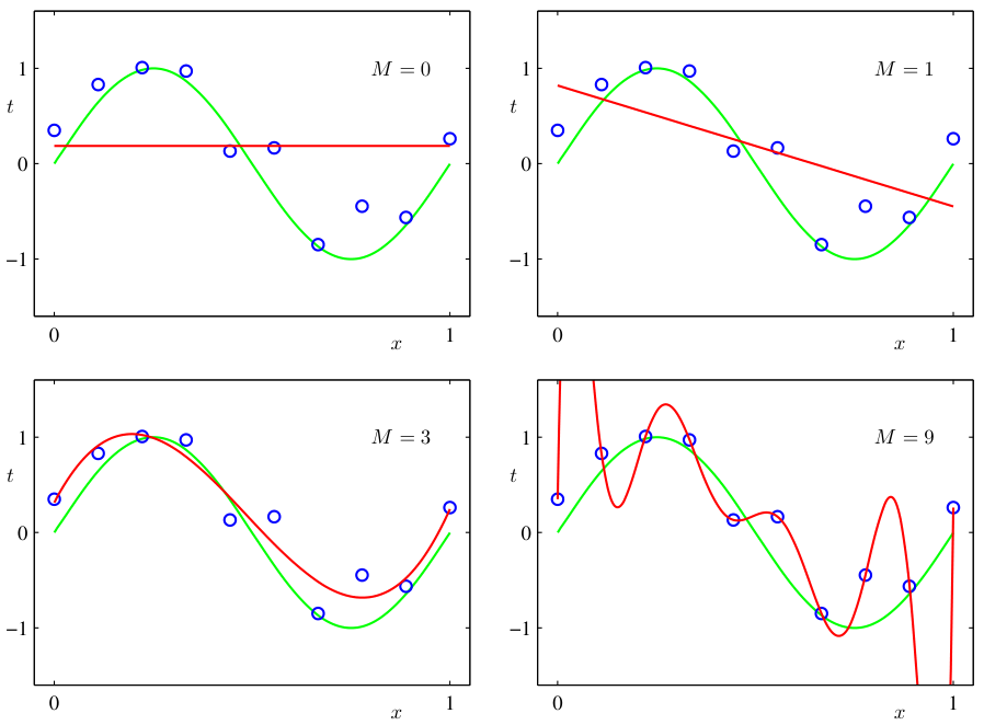
Overfitting — definition and visual example

Overfitting: the model captures noise and idiosyncrasies of the training data instead of the underlying signal.
Symptom: training error is very low, test error is high.
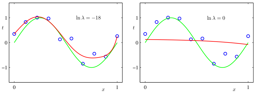
Visual: a high-degree polynomial passes through every training point but oscillates wildly between them.
M = 9 (bottom right) has zero training error but wild oscillations everywhere else.

Polynomial fits of degree M = 0, 1, 3, 9 to N = 10 noisy points. The degree-9 fit is a textbook example of overfitting [@bishop2006pattern, Fig. 1.4].

Underfitting — definition and visual example

Underfitting: the model is too simple to capture the structure in the data.
Symptom: both training and test error are high.
Visual: a straight line fit to clearly nonlinear data misses the pattern entirely.

The complexity spectrum

Low complexity (few parameters, simple model): high bias, low variance → underfitting.
High complexity (many parameters, flexible model): low bias, high variance → overfitting.
The sweet spot: enough complexity to capture the signal, not so much that it captures noise.

Interactive: The Complexity Spectrum

//| echo: false
//| panel: input
viewof polyDegree = Inputs.range([1, 15], {value: 1, step: 1, label: "Polynomial Degree (Complexity)"})

Training Data: 15 samples Noise: $\sigma = 0.2$

//| echo: false
html`
<div style="margin-top: 20px;">
  <strong>Train MSE:</strong> ${mse.train.toFixed(3)}<br>
  <strong>Test MSE:</strong> ${mse.test.toFixed(3)}
</div>
`

//| echo: false
d3 = require("d3@7")
d3_reg = require("d3-regression@1")
seed = 42
randomVal = d3.randomNormal.source(d3.randomLcg(seed))(0, 0.2)
trueFunc = (x) => Math.sin(1.5 * Math.PI * x)

points = {
  const train = Array.from({length: 15}, (_, i) => {
    let x = (i+0.5) / 15 + (d3.randomUniform.source(d3.randomLcg(seed+i))() - 0.5) * 0.05;
    return {x: x, y: trueFunc(x) + randomVal(), type: "train"};
  });
  const test = Array.from({length: 100}, (_, i) => {
    let x = (i+0.5) / 100;
    return {x: x, y: trueFunc(x) + randomVal(), type: "test"};
  });
  return [...train, ...test];
}

trainPts = points.filter(d => d.type === "train")
testPts = points.filter(d => d.type === "test")

polyModel = {
  try {
    return d3_reg.regressionPoly().x(d => d.x).y(d => d.y).order(polyDegree)(trainPts);
  } catch(e) {
    // fallback if d3-regression fails for very high degrees/collinearity
    return {predict: (x) => 0}; 
  }
}

mse = {
  const trainMSE = d3.mean(trainPts, d => Math.pow(polyModel.predict(d.x) - d.y, 2));
  const testMSE = d3.mean(testPts, d => Math.pow(polyModel.predict(d.x) - d.y, 2));
  return {train: trainMSE || 0, test: testMSE || 0};
}

Plot.plot({
  width: 1000,
  height: 600,
  y: {domain: [-2, 2], grid: true},
  x: {domain: [0, 1], grid: true},
  color: {domain: ["train", "test"], range: ["red", "steelblue"]},
  marks: [
    Plot.dot(points, {x: "x", y: "y", fill: "type", fillOpacity: 0.8, r: d => d.type === "train" ? 6 : 3}),
    Plot.line(d3.range(0, 1.01, 0.01), {x: d => d, y: d => trueFunc(d), stroke: "gray", strokeDasharray: "4,4", strokeWidth: 2, title: "True Function"}),
    Plot.line(d3.range(0, 1.01, 0.01).map(x => ({x: x, y: polyModel.predict(x)})), {x: "x", y: "y", stroke: "orange", strokeWidth: 4, title: "Fitted Model", clip: true})
  ]
})

Detecting overfitting in practice

Plot training loss and validation loss over training epochs.
Healthy: both decrease and converge.
Overfitting: training loss continues to decrease while validation loss starts increasing.
The divergence point suggests when to stop training (early stopping) [@neuer2024machine].

Train vs test RMS error as a function of polynomial order M. Low M → underfitting; M = 9 → test error explodes [@bishop2006pattern, Fig. 1.5].

Overfitting boundary in a classification setting [@neuer2024machine, Fig. 4.8]: the overfit boundary memorizes noise and fails to generalize.

Engineering consequence: false confidence

A model with 99% training accuracy may have 60% test accuracy.
In materials science: a property-prediction model that overfits may suggest alloy compositions that fail experimentally.
Perfect training fit can mask catastrophic deployment failure — always validate on held-out data.

Setup: expected prediction error

Consider the expected loss over both the training data $\mathcal{D}$ and a new test point $(\mathbf{x}, y)$:

\[ \text{EPE}(\mathbf{x}) = \mathbb{E}_{\mathcal{D}} \mathbb{E}_{y|\mathbf{x}} \big[ (y - \hat{f}_{\mathcal{D}}(\mathbf{x}))^2 \big] \]

This averages over all possible training sets and all possible true outputs at $\mathbf{x}$.

Decomposing squared error — step 1

Add and subtract the expected prediction $\mathbb{E}_{\mathcal{D}}[\hat{f}(\mathbf{x})]$:

\[ y - \hat{f}(\mathbf{x}) = \underbrace{(y - f(\mathbf{x}))}_{\text{noise}} + \underbrace{(f(\mathbf{x}) - \mathbb{E}_{\mathcal{D}}[\hat{f}(\mathbf{x})])}_{\text{bias}} + \underbrace{(\mathbb{E}_{\mathcal{D}}[\hat{f}(\mathbf{x})] - \hat{f}(\mathbf{x}))}_{\text{variance term}} \]

Decomposing squared error — step 2

Square the expression and take expectations.

Cross-terms vanish because noise is independent of the model and $\mathbb{E}_{\mathcal{D}}[\hat{f}(\mathbf{x}) - \mathbb{E}_{\mathcal{D}}[\hat{f}(\mathbf{x})]] = 0$.

The three surviving terms give us the decomposition.

The three components

\[ \text{EPE}(\mathbf{x}) = \underbrace{\sigma^2_{\text{noise}}}_{\text{irreducible}} + \underbrace{\big(\mathbb{E}_{\mathcal{D}}[\hat{f}(\mathbf{x})] - f(\mathbf{x})\big)^2}_{\text{Bias}^2} + \underbrace{\mathbb{E}_{\mathcal{D}}\big[(\hat{f}(\mathbf{x}) - \mathbb{E}_{\mathcal{D}}[\hat{f}(\mathbf{x})])^2\big]}_{\text{Variance}} \]

Bias²: systematic error from model assumptions.
Variance: sensitivity to the specific training set.
Noise: irreducible — the Bayes error [@bishop2006pattern].

Bias — interpretation

Bias measures how far the average prediction (over all possible training sets) is from the truth.
High bias means the model class cannot represent the true function.
Example: fitting a linear model to quadratic data — no amount of data will fix the systematic error.
Bias is a property of the model family, not the specific training set.

Variance — interpretation

Variance measures how much the prediction changes when we draw a different training set.
High variance means the model is too sensitive to the particular data it was trained on.
Example: a degree-15 polynomial changes dramatically with each new training sample.
Variance is controlled by model complexity and training set size.

Intrinsic noise / Bayes error

The noise term $\sigma^2$ represents inherent randomness in the data-generating process.
No model — no matter how complex — can reduce the error below this floor.
In materials science: measurement noise, batch-to-batch variability, uncontrolled environmental factors.
Estimating $\sigma^2$ helps set realistic performance expectations.

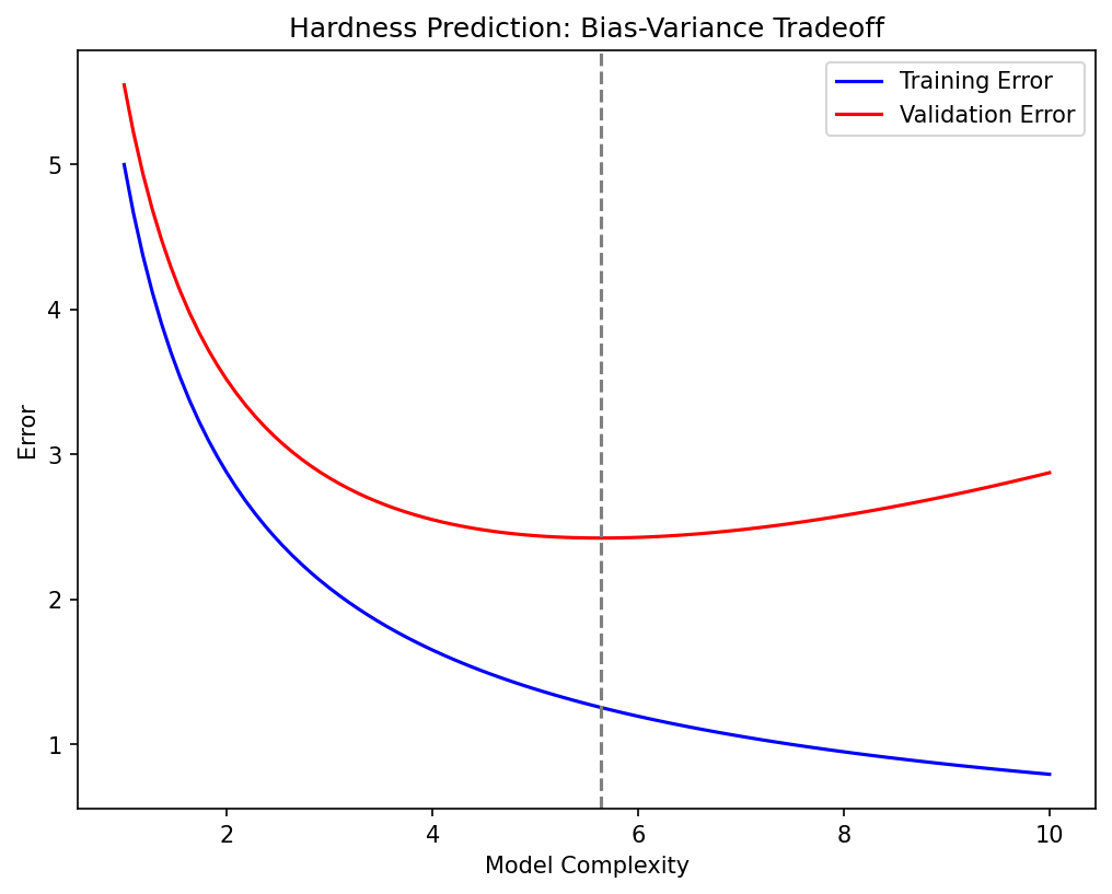
The bias-variance tradeoff

Increasing complexity: bias decreases (model can fit more patterns), variance increases (model fits noise too).
Decreasing complexity: variance decreases (model is stable), bias increases (model misses structure).
Optimal complexity minimizes the sum Bias² + Variance.
This is the most fundamental tradeoff in machine learning [@murphy2012machine].

High-bias (top) vs high-variance (bottom) regime visualised by 20 fitted curves and their mean (red) vs the true function (green). [@murphy2012machine, Fig. 6.5] (based on [@bishop2006pattern, Fig. 3.5])

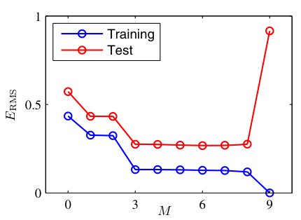
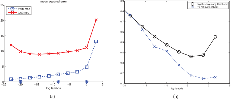
Visual: U-shaped total error curve — from data

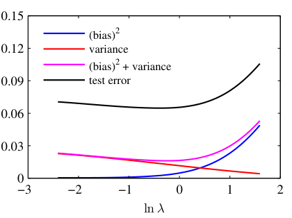
Bias², variance, and their sum vs regularization strength ln(λ). The minimum of Bias² + Variance (≈ ln λ = −0.31) closely matches the test-set error minimum — the operational sweet spot [@bishop2006pattern, Fig. 3.6].

Visual: U-shaped total error curve — schematic

%%| echo: false
%%| fig-align: center
%%| align: center
graph LR
    C["Model Complexity"] --> B["Bias decreases"]
    C --> V["Variance increases"]
    B --> E["Total Error"]
    V --> E
    N["Noise"] --> E
    style E fill:#f9f,stroke:#333,stroke-width:4px
    style C fill:#ccf,stroke:#333

Plot Bias², Variance, and total error against model complexity.
Bias² decreases monotonically with complexity.
Variance increases monotonically with complexity.
Total error = Bias² + Variance + noise: a U-shaped curve with a minimum at optimal complexity.

Modern view: double descent

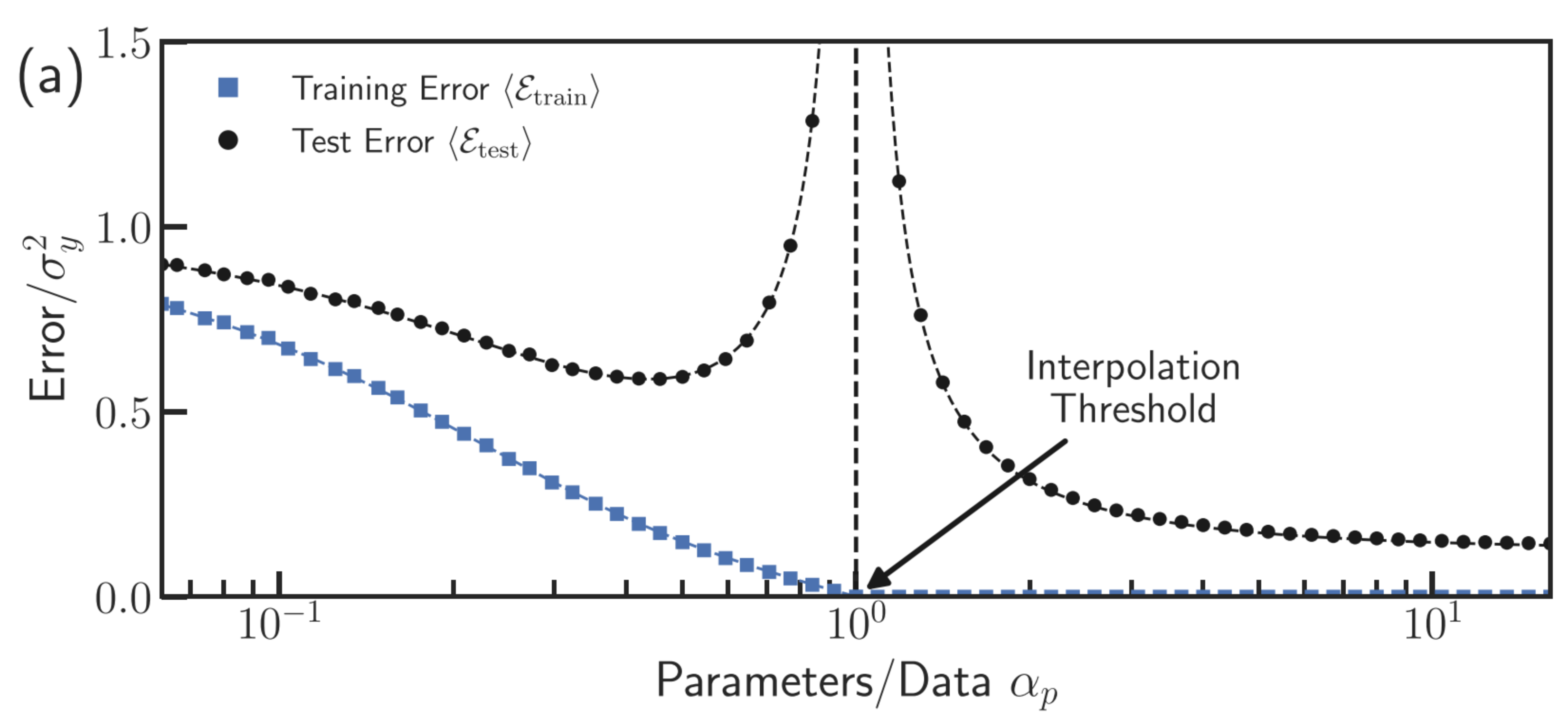
Classical theory predicts a U-shaped test error curve: error falls, then rises with model complexity.
Modern overparameterized models (deep neural networks) show a second descent: beyond the interpolation threshold, test error falls again.
The interpolation threshold occurs when the number of parameters equals the number of training points.
Beyond the threshold, the model is expressive enough to interpolate — but the minimum-norm solution generalizes well [@belkin2019reconciling; @nakkiran2020deep].

Double descent in a two-layer neural network: training error (blue squares) falls to zero at the interpolation threshold, while test error (black circles) peaks then decreases again in the overparameterized regime [@rocks2022memorizing].

Interactive: Bias and Variance Demystified

//| echo: false
//| panel: input
viewof bvDegree = Inputs.range([1, 12], {value: 3, step: 1, label: "Model Complexity (Degree)"})
viewof numSamples = Inputs.range([5, 50], {value: 10, step: 5, label: "Number of Datasets"})
viewof showAverage = Inputs.toggle({label: "Show Expected Fit (Bias)", value: false})

Each faint blue curve is trained on a different dataset sampled from the true distribution.
The spread of these curves represents Variance.
The distance from the red average curve to the true function represents Bias.

//| echo: false
bvDatasets = {
  const sets = [];
  for(let i=0; i<numSamples; i++) {
    const rng = d3.randomNormal.source(d3.randomLcg(seed * 10 + i))(0, 0.4);
    const pts = Array.from({length: 12}, (_, j) => {
      let x = (j+0.5)/12 + (d3.randomUniform.source(d3.randomLcg(seed * 100 + i*12 + j))() - 0.5) * 0.05;
      return {x: x, y: trueFunc(x) + rng()};
    });
    sets.push(pts);
  }
  return sets;
}

bvModels = bvDatasets.map(pts => d3_reg.regressionPoly().x(d=>d.x).y(d=>d.y).order(bvDegree)(pts))

bvLines = bvModels.flatMap((model, i) => {
  return d3.range(0, 1.05, 0.05).map(x => ({x: x, y: model.predict(x), lineId: i, type: "individual"}));
})

bvAverageLine = {
  const xs = d3.range(0, 1.05, 0.05);
  return xs.map(x => {
    const sum = bvModels.reduce((acc, m) => acc + m.predict(x), 0);
    return {x: x, y: sum / numSamples, type: "average"};
  });
}

Plot.plot({
  width: 1000,
  height: 600,
  y: {domain: [-2, 2], grid: true},
  x: {domain: [0, 1], grid: true},
  marks: [
    Plot.line(d3.range(0, 1.01, 0.01), {x: d => d, y: d => trueFunc(d), stroke: "gray", strokeDasharray: "4,4", strokeWidth: 3, title: "True Function"}),
    Plot.line(bvLines, {x: "x", y: "y", z: "lineId", stroke: "steelblue", strokeOpacity: 0.2, strokeWidth: 2, clip: true}),
    showAverage ? Plot.line(bvAverageLine, {x: "x", y: "y", stroke: "red", strokeWidth: 5, strokeDasharray: "2,2", title: "Average Fit", clip: true}) : null
  ]
})

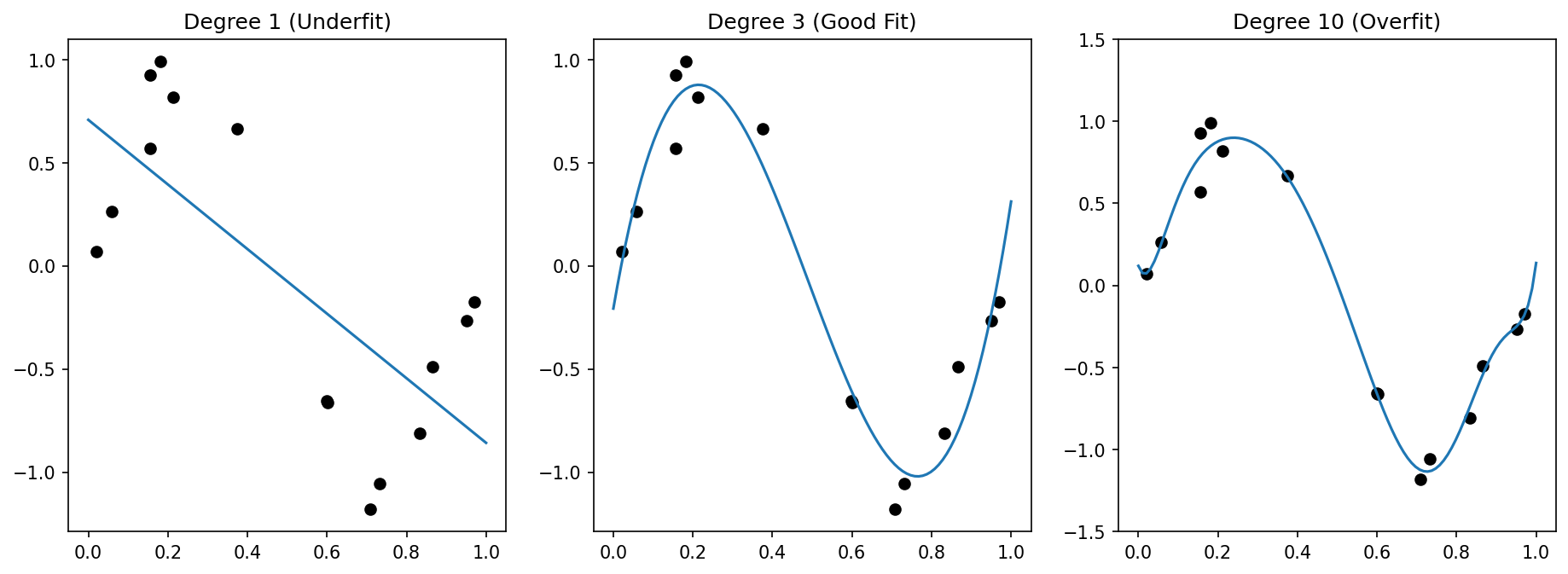
Example: polynomial regression

Degree 1: high bias (line cannot capture curvature), low variance → underfitting.
Degree 3–5: moderate bias and variance → good fit.
Degree 15: low bias (passes through training points), high variance (oscillates wildly) → overfitting.
The optimal degree depends on the data: amount of noise, sample size, true function complexity.

L = 100 datasets fitted with different regularization strengths. Left column: individual fits. Right column: ensemble mean vs true sinusoid. High λ → low variance, high bias (top); low λ → high variance, low bias (bottom). [@bishop2006pattern, Fig. 3.5]

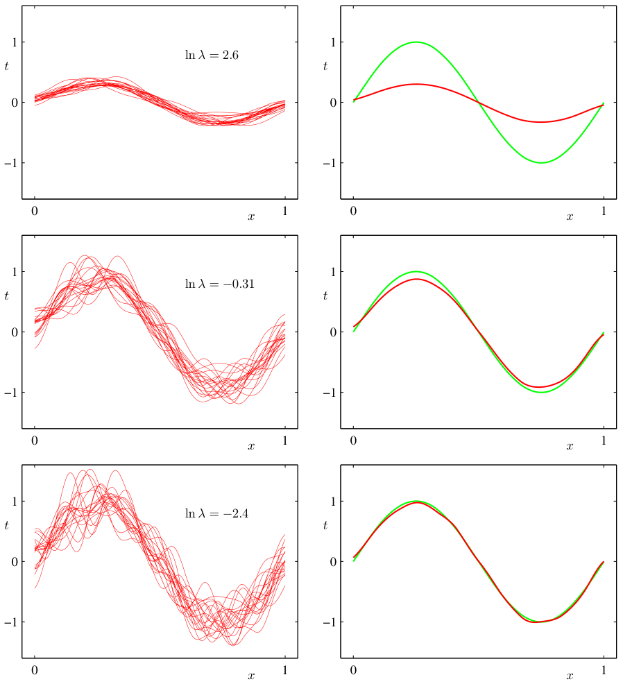
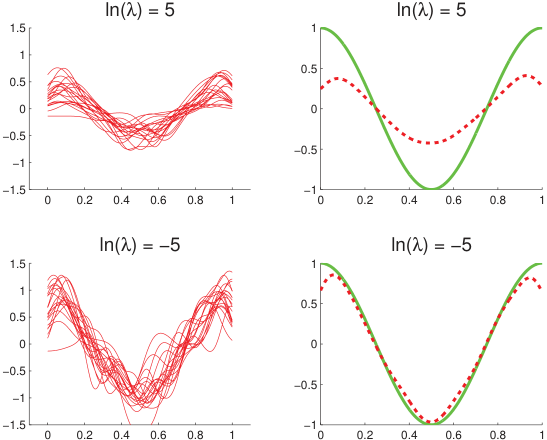
Example: Ridge regression and the tradeoff

Ridge regression with regularization parameter $\lambda$:
- High $\lambda$: heavy shrinkage → high bias, low variance.
- Low $\lambda$: minimal shrinkage → low bias, high variance.
$\lambda$ acts as a complexity knob that traces out the bias-variance tradeoff.
Optimal $\lambda$ minimizes total MSE, not training error [@murphy2012machine].

Degree-14 polynomial with increasing L2 regularization. Left (λ ≈ 0): wiggly overfit. Right (large λ): over-smoothed. Stars mark the same λ values as in Figure 7.8. [@murphy2012machine, Fig. 7.7]

Checkpoint: why is the MLE not always best?

Maximum Likelihood Estimation is unbiased but can have high variance.
A biased estimator (MAP / regularized) can achieve lower total MSE.
The key insight: introducing a small bias can yield a large variance reduction.
This is the mathematical justification for regularization.

Regularization — the key idea

Add a penalty to the loss function that discourages unnecessary complexity:

\[ J_{\text{reg}}(\mathbf{w}) = \underbrace{\frac{1}{N}\sum_{i=1}^{N} L(\hat{y}_i, y_i)}_{\text{data fit}} + \underbrace{\lambda \cdot \Omega(\mathbf{w})}_{\text{complexity penalty}} \]

The penalty $\Omega(\mathbf{w})$ grows with model complexity.
$\lambda > 0$ controls the strength of regularization.

Regularized ERM

The regularized optimization problem:

\[ \hat{\mathbf{w}} = \arg\min_{\mathbf{w}} \left[ R_N(\mathbf{w}) + \lambda \, \Omega(\mathbf{w}) \right] \]

$\lambda = 0$: no regularization (pure ERM).
$\lambda \to \infty$: penalty dominates — model collapses to the simplest possible solution.
Choosing $\lambda$ is a model selection problem, not a parameter estimation problem.

Ridge regression (L2 penalty)

Penalty: $\Omega(\mathbf{w}) = \|\mathbf{w}\|_2^2 = \sum_j w_j^2$.
Loss:

\[ L_{\text{ridge}} = \sum_{i=1}^{N}(\hat{y}_i - y_i)^2 + \lambda \|\mathbf{w}\|_2^2 \]

Effect: shrinks all coefficients toward zero, but none exactly to zero.
Equivalent to a Gaussian prior on weights in Bayesian interpretation.

Ridge regression — closed-form solution

\[ \hat{\mathbf{w}}_{\text{ridge}} = (\mathbf{X}^\top\mathbf{X} + \lambda\mathbf{I})^{-1}\mathbf{X}^\top\mathbf{y} \]

Adding $\lambda\mathbf{I}$ makes the matrix always invertible (even if $\mathbf{X}^\top\mathbf{X}$ is singular).
This stabilizes the solution when features are correlated or $p > N$.
The closed form connects regularization directly to linear algebra [@mcclarren2021machine].

Effect of regularization strength on an M = 9 polynomial. ln λ = −18 (left) suppresses overfitting; ln λ = 0 (right) over-shrinks. [@bishop2006pattern, Fig. 1.7]

Ridge circular constraint [@mcclarren2021machine, Fig. 2.7]: The LS unconstrained optimum is outside the circle; the ridge solution (star) lands on the boundary.

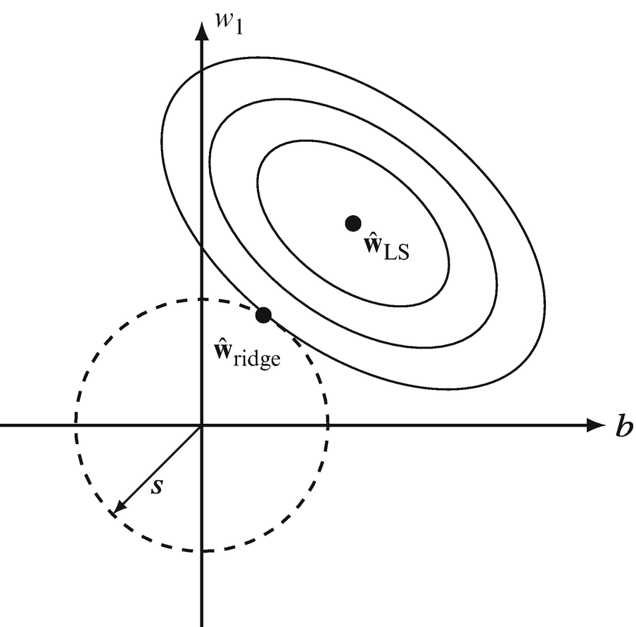
Ridge regression — geometric view

The unconstrained optimum lies at the OLS solution.
Ridge constrains the solution to lie within a sphere $\|\mathbf{w}\|_2^2 \leq t$.
The regularized solution is the point on the sphere closest to the OLS solution.
Contour plot: elliptical loss contours intersect the circular constraint region.

Ridge (circle, left) vs Lasso (diamond, right) constraint regions with OLS error ellipses. The lasso solution lands at a corner, setting w₁* = 0 exactly. [@bishop2006pattern, Fig. 3.4]

Lasso regression (L1 penalty)

Penalty: $\Omega(\mathbf{w}) = \|\mathbf{w}\|_1 = \sum_j |w_j|$.
Loss:

\[ L_{\text{lasso}} = \sum_{i=1}^{N}(\hat{y}_i - y_i)^2 + \lambda \|\mathbf{w}\|_1 \]

Key property: Lasso can set coefficients exactly to zero — it performs variable selection.

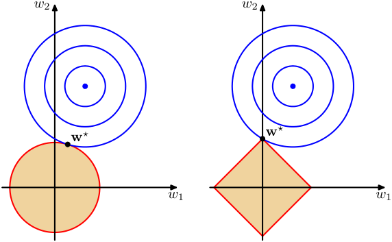
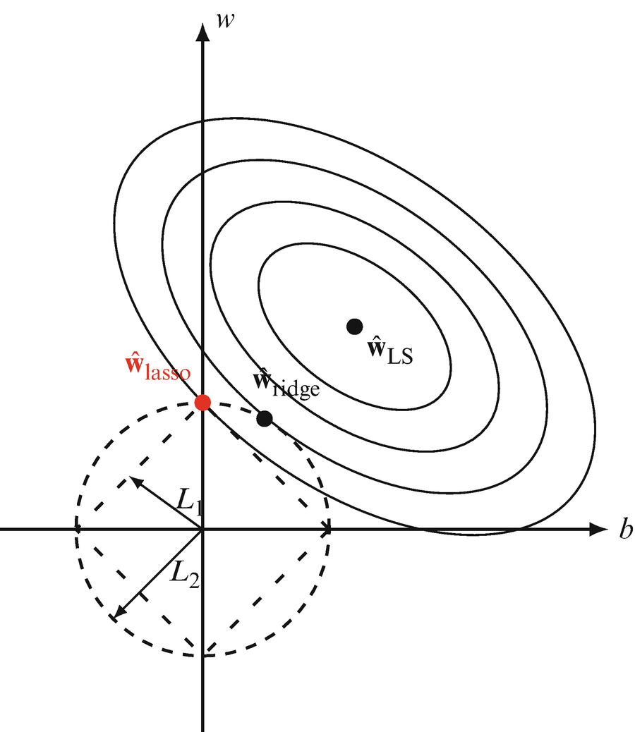
Lasso — geometric view and sparsity

The L1 constraint region is a diamond (in 2D) or cross-polytope (in higher dimensions).
The diamond has corners that lie on coordinate axes.
Loss contours are more likely to intersect a corner → some coefficients become exactly zero.
This geometric property is why L1 promotes sparsity while L2 does not [@mcclarren2021machine].

Lasso diamond constraint [@mcclarren2021machine, Fig. 2.8]: The elliptic error contours touch the diamond at a corner — one coefficient is exactly zero, producing a sparse solution.

Interactive Geometry: Ridge vs Lasso

//| echo: false
//| panel: input
viewof regType = Inputs.radio(["Lasso (L1)", "Ridge (L2)"], {value: "Lasso (L1)", label: "Regularization Type"})
viewof constraintT = Inputs.range([0.1, 3], {value: 1.5, step: 0.05, label: "Constraint Bound (t)"})

A geometric view of minimizing $MSE(\mathbf{w})$ subject to $\Omega(\mathbf{w}) \leq t$.
In the dual, a smaller $t$ corresponds to a larger $\lambda$.
Notice how the optimal regularized solution (red dot) naturally strikes the corners of the L1 diamond, setting $w_2=0$ identically.

//| echo: false

constraintRegion = {
  if (regType === "Ridge (L2)") {
    return d3.range(0, 2 * Math.PI + 0.1, 0.1).map(theta => {
      const r = constraintT;
      return {w1: r * Math.cos(theta), w2: r * Math.sin(theta)};
    });
  } else {
    return [
      {w1: constraintT, w2: 0},
      {w1: 0, w2: constraintT},
      {w1: -constraintT, w2: 0},
      {w1: 0, w2: -constraintT},
      {w1: constraintT, w2: 0}
    ];
  }
}

minPointPerfect = {
  const unconstrainedLoss = 0; 
  let inRegion = false;
  if (regType === "Ridge (L2)") {
    inRegion = (2*2 + 1*1) <= constraintT*constraintT;
  } else {
    inRegion = (2 + 1) <= constraintT;
  }
  
  if (inRegion) return {w1: 2, w2: 1};

  let minLoss = Infinity;
  let bestW1 = 0, bestW2 = 0;
  
  if (regType === "Ridge (L2)") {
    for (let theta = 0; theta < 2*Math.PI; theta += 0.01) {
      let w1 = constraintT * Math.cos(theta);
      let w2 = constraintT * Math.sin(theta);
      let loss = Math.pow(w1 - 2, 2) + 3 * Math.pow(w2 - 1, 2);
      if (loss < minLoss) { minLoss = loss; bestW1 = w1; bestW2 = w2; }
    }
  } else {
    const segments = [
      {sw1: constraintT, sw2: 0, ew1: 0, ew2: constraintT},
      {sw1: 0, sw2: constraintT, ew1: -constraintT, ew2: 0},
      {sw1: -constraintT, sw2: 0, ew1: 0, ew2: -constraintT},
      {sw1: 0, sw2: -constraintT, ew1: constraintT, ew2: 0}
    ];
    for (const seg of segments) {
      for (let alpha = 0; alpha <= 1; alpha += 0.005) {
        let w1 = seg.sw1 * (1 - alpha) + seg.ew1 * alpha;
        let w2 = seg.sw2 * (1 - alpha) + seg.ew2 * alpha;
        let loss = Math.pow(w1 - 2, 2) + 3 * Math.pow(w2 - 1, 2);
        if (loss < minLoss) { minLoss = loss; bestW1 = w1; bestW2 = w2; }
      }
    }
  }
  
  if (regType === "Lasso (L1)") {
     if (Math.abs(bestW1) < 0.05) { bestW1 = 0; bestW2 = constraintT * Math.sign(bestW2); }
     if (Math.abs(bestW2) < 0.05) { bestW2 = 0; bestW1 = constraintT * Math.sign(bestW1); }
  }
  
  return {w1: bestW1, w2: bestW2};
}

contourLines = {
  const lines = [];
  const minLoss = Math.pow(minPointPerfect.w1 - 2, 2) + 3 * Math.pow(minPointPerfect.w2 - 1, 2);
  const levels = [0.5, 2, 4, 8, 12, minLoss];
  for (const C of levels) {
    if (C < 0) continue;
    const pts = [];
    for (let alpha = 0; alpha <= 2*Math.PI + 0.1; alpha += 0.05) {
      pts.push({
        w1: 2 + Math.sqrt(C) * Math.cos(alpha),
        w2: 1 + Math.sqrt(C/3) * Math.sin(alpha),
        level: C,
        isMin: Math.abs(C - minLoss) < 0.01
      });
    }
    lines.push(pts);
  }
  return lines;
}

Plot.plot({
  width: 800,
  height: 600,
  x: {domain: [-2, 3], grid: true, label: "Coefficient w1"},
  y: {domain: [-2, 3], grid: true, label: "Coefficient w2"},
  marks: [
    ...contourLines.map(pts => 
      Plot.line(pts, {x: "w1", y: "w2", stroke: d => d.isMin[0] ? "red" : "gray", strokeWidth: d => d.isMin[0] ? 3 : 1})
    ),
    Plot.line(constraintRegion, {x: "w1", y: "w2", stroke: "steelblue", fill: "steelblue", fillOpacity: 0.2, strokeWidth: 2}),
    Plot.dot([minPointPerfect], {x: "w1", y: "w2", fill: "red", r: 8}),
    Plot.dot([{w1: 2, w2: 1}], {x: "w1", y: "w2", fill: "black", r: 5, stroke: "white"}),
    Plot.text([{w1: 2, w2: 1.15}], {x: "w1", y: "w2", text: () => "OLS Unconstrained Min", fill: "black"})
  ]
})

Ridge vs Lasso — side-by-side comparison

Property	Ridge (L2)	Lasso (L1)
Penalty	$\sum w_j^2$	$\sum \\|w_j\\|$
Sparsity	No (shrinks all)	Yes (zeroes some)
Closed form	Yes	No (requires optimization)
Correlated features	Keeps all, shrinks equally	Selects one arbitrarily
Best for	Many relevant features	Few relevant features

Ridge: Shrinks coefficients toward zero, stabilizes solutions.
Lasso: Zeroes out coefficients, performs feature selection.
Guideline: Use Lasso if you expect a sparse underlying signal [@mcclarren2021machine].

Elastic net (brief)

Combines L1 and L2 penalties:

\[ \Omega(\mathbf{w}) = \alpha \|\mathbf{w}\|_1 + (1 - \alpha) \|\mathbf{w}\|_2^2 \]

Gets sparsity from L1 and stability from L2.
Handles correlated feature groups better than pure Lasso.
$\alpha$ interpolates between Ridge ($\alpha = 0$) and Lasso ($\alpha = 1$).

Normalization requirement

Regularization penalizes coefficient magnitude.
If features have different scales, the penalty is inconsistent: large-scale features get penalized more.
Always normalize/standardize features before applying regularization.
Standard approach: zero mean, unit variance for each feature [@mcclarren2021machine].

Dropout as regularization (neural networks)

During training, randomly set each neuron’s output to zero with probability $p$.
Effect: the network cannot rely on any single neuron → prevents co-adaptation.
At test time, scale activations by $(1-p)$ to compensate.
Dropout is equivalent to training an ensemble of $2^H$ sub-networks (where $H$ = number of hidden units).

Choosing lambda — preview of cross-validation

$\lambda$ is a hyperparameter — it controls model complexity but is not a model parameter.
It cannot be learned from training data alone (that would just lead to $\lambda = 0$).
We need a principled method to select $\lambda$: cross-validation.

Train / validation / test — the three roles

Training set: used to fit model parameters $\mathbf{w}$.
Validation set: used to tune hyperparameters ($\lambda$, architecture, learning rate).
Test set: used once for final performance evaluation — never used during development.
Typical split: 60% train / 20% validation / 20% test.

Why we need three sets, not two

If we use the test set to select $\lambda$, the reported test performance is optimistically biased.
The test set must remain untouched until the very end.
The validation set absorbs the selection bias instead.
Violation of this principle is one of the most common mistakes in applied ML.

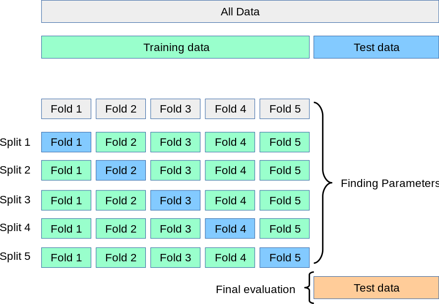
k-fold cross-validation — procedure

Split data into $k$ equal folds.
For each fold $j = 1, \dots, k$:
- Train on all folds except fold $j$.
- Evaluate on fold $j$.
Average the $k$ performance estimates:

\[ \text{CV}(k) = \frac{1}{k} \sum_{j=1}^{k} R_{\text{test}}^{(j)} \]

Common choice: $k = 5$ or $k = 10$ [@neuer2024machine].

5-fold cross-validation: training data is split into 5 folds; each fold serves once as the validation set while the model trains on the remaining four. The held-out test set is used only for final evaluation [@scikit-learn].

k-fold cross-validation — variance reduction

Every data point is used for both training and evaluation (in different folds).
More efficient use of limited data compared to a single train/validation split.
The averaged estimate has lower variance than a single hold-out estimate.
Tradeoff: $k$ times more expensive computationally.

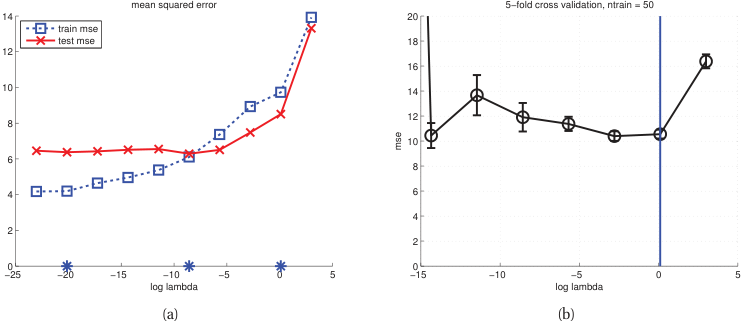
Choosing lambda via CV

For each candidate $\lambda$, compute the CV error $\text{CV}(\lambda)$.
Plot $\text{CV}(\lambda)$ vs $\log(\lambda)$.
Select $\lambda^*$ at the minimum of the CV curve.
The one-standard-error rule: pick the simplest model within one SE of the minimum [@murphy2012machine].

Train MSE (dashed blue) and test MSE (solid red) vs log(λ) for ridge-regularized degree-14 polynomial. Right of minimum = underfit. Left of minimum = overfit. [@murphy2012machine, Fig. 7.8a]

5-fold CV error vs log(λ) with one-SE rule (blue line) for selecting a parsimonious λ. [@murphy2012machine, Fig. 6.6b]

Model selection: complexity vs performance

Cross-validation is not limited to tuning $\lambda$.
Compare entirely different model families: linear, polynomial, neural network, random forest.
For each model, tune its hyperparameters via inner CV loop.
Select the model family with the best outer CV performance.

Checkpoint MCQ slide

Scenario: A student uses the test set to tune $\lambda$, then reports test set accuracy as the model’s generalization performance. What goes wrong?
1. Nothing — this is standard practice.
1. The reported accuracy is pessimistically biased.
1. The reported accuracy is optimistically biased.
1. The model will underfit.
Answer: C — the test set was used for selection, so it no longer provides an unbiased estimate.

Materials example: overfitting in alloy property prediction

Setting: predicting hardness from 50 compositional features using only 200 samples.
Without regularization: the model memorizes training data and predicts poorly on new alloys.
With Ridge regularization ($\lambda$ selected via 5-fold CV): test error drops by 40%.
Lesson: when $p/N$ is large, regularization is not optional — it is essential.

Hardness prediction error vs model complexity.

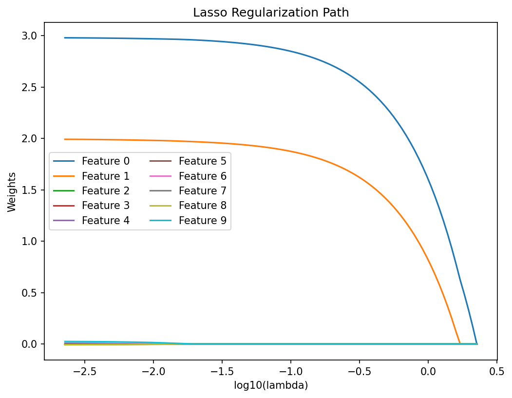
Materials example: Lasso for identifying governing features

Starting from 100 candidate features (composition, processing, microstructure).
Lasso with increasing $\lambda$ progressively zeros out irrelevant features.
The surviving features align with known physical mechanisms (grain size, carbon content, cooling rate).
Lasso provides both prediction and interpretability.

Lasso coefficient paths vs regularization strength.

Materials example: polynomial models for process-property curves

A high-degree polynomial captures batch-to-batch noise in sintering temperature vs density data.
A low-degree polynomial misses the genuine nonlinearity (plateau near full density).
Cross-validation identifies degree 3 as the sweet spot for this dataset.
This is the bias-variance tradeoff in action on real engineering data.

Comparison of underfitting, good fit, and overfitting.

Trees, forests, and boosting — where they fit

We just spent the unit on bias-variance decomposition and regularization.
Two practical model families are best understood directly through this lens:
- Random Forests = variance reduction by averaging.
- Gradient Boosting = bias reduction by sequential refinement.
For tabular materials data, these usually beat neural networks. Knowing them well is non-negotiable for a working materials engineer.

Decision trees — a single learner

A decision tree partitions input space by axis-aligned splits.

Internal node: a test like “Cr fraction $> 0.18$?”
Leaf: a constant prediction (mean for regression, majority class for classification).
Prediction: route a new $x$ down the tree to its leaf.

Trees are non-parametric: capacity grows with depth.
Naturally handle mixed feature types (continuous, categorical, binary).
No normalization needed — splits are scale-invariant.

How splits are chosen

At each node, choose the feature and threshold that maximize impurity reduction:

\[ \Delta = I(\text{parent}) - \frac{N_L}{N} I(\text{left}) - \frac{N_R}{N} I(\text{right}). \]

Regression: $I = $ within-node variance (squared-error reduction).
Classification: $I = $ Gini impurity $\sum_c p_c (1 - p_c)$ or entropy $-\sum_c p_c \log p_c$.
The split search is greedy — best split at each node, no backtracking.

A single tree is a high-variance learner

Stop splitting too early → underfit (high bias, low variance).
Grow to pure leaves → fits training data perfectly (low bias, high variance).
A small change in training data can completely reshape a deep tree.
Pruning helps but is fragile.

This is exactly the regime where averaging helps. Cue ensembles.

Bagging — variance reduction by averaging

Bootstrap aggregating [@breiman1996bagging]:

Draw $B$ bootstrap samples from the training data (sample with replacement, same size $N$).
Train one tree per bootstrap sample (no pruning, fully grown).
Average their predictions: $\hat f_{\text{bag}}(x) = \frac{1}{B}\sum_{b=1}^B \hat f_b(x)$.

\[\mathrm{Var}\!\left(\frac{1}{B}\sum_b \hat f_b\right) = \frac{\sigma^2}{B} + \rho\!\left(1 - \frac{1}{B}\right)\sigma^2.\]

Variance shrinks as $B$ grows — but only as fast as tree-pair correlation $\rho$ allows.

Random forest = bagging + random feature subsets

At each split, search only a random subset of features (typical: $\sqrt{d}$ for classification, $d/3$ for regression).
This decorrelates the trees: $\rho \downarrow$, so the variance reduction from averaging is much larger.
All other tree mechanics unchanged.
Default in scikit-learn: RandomForestRegressor, RandomForestClassifier [@breiman2001randomforests].

Performance: with $B = 500$ trees and reasonable feature subsetting, RF usually beats a tuned single tree by a wide margin.

Random forest in practice

Out-of-bag (OOB) error: each bootstrap sample omits ~37% of training data; predict on those for a free CV-like estimate.
Feature importance: aggregate the impurity reduction each feature contributes across all splits in all trees.
Hyperparameters that matter: number of trees ($B$), min samples per leaf, max features per split.
Hyperparameters that mostly don’t: tree depth (let them grow), splitting criterion.

Boosting — sequential bias reduction

Bagging averages many low-bias, high-variance learners → reduces variance.
Boosting does the opposite: it builds a sequence of high-bias, low-variance learners (shallow trees, “weak learners”), each correcting the residual error of the previous ensemble.
$\hat f^{(t)}(x) = \hat f^{(t-1)}(x) + \eta \cdot h_t(x)$.
Result: bias decreases as the ensemble grows.

Where bagging averages independent learners, boosting composes dependent learners.

Gradient boosting — fit the negative gradient

For loss $\mathcal{L}$, at iteration $t$:

Compute pseudo-residuals: $r_i^{(t)} = -\partial \mathcal{L}(y_i, \hat f^{(t-1)}(x_i)) / \partial \hat f^{(t-1)}(x_i)$.
Fit a small tree $h_t$ to predict the residuals.
Update: $\hat f^{(t)} = \hat f^{(t-1)} + \eta \cdot h_t$.

$\eta$: learning rate (shrinkage). Small $\eta$ + many trees > large $\eta$ + few trees.

XGBoost, LightGBM, CatBoost

The 2025 toolbox for tabular data:

XGBoost [@chen2016xgboost]: gradient boosting + L2 regularization on leaf values + histogram-based splits + careful missing-value handling.
LightGBM: faster on large datasets via leaf-wise growth and gradient-based one-side sampling.
CatBoost: best out-of-box on heavy categorical features (alloy chemistries, processing routes).
All three: drop-in scikit-learn-compatible, support GPU, handle missing values natively.

Practical advice: XGBoost is the default; LightGBM if $N > 10^6$; CatBoost if you have lots of categorical features.

Trees vs neural networks on tabular data

Trees / boosting win when:

Tabular features (compositions, parameters).
$N < 10^5$ rows.
Mixed feature types.
Strong feature interactions, weak structure.
You want fast training and feature importance.

Neural networks win when:

Spatial / sequential / graph data.
$N \gg 10^5$ rows.
Pre-trained foundation models exist (Unit 9).
End-to-end pipelines from raw signals.

For most materials projects with tabular features, try gradient boosting first. Use a NN only if the data shape demands it.

Watch for: TabPFN [@hollmann2023tabpfn] — a transformer pre-trained on synthetic tabular tasks that does zero-shot classification by passing the entire training set as a context window. As of 2025, competitive with XGBoost on small ($\leq 10\text{k}$ rows) tabular benchmarks. Not a replacement at scale, but the first credible deep-learning approach to tabular data.

Materials example — alloy property prediction

Dataset: 5000 alloys, 12 elemental fractions + 4 processing parameters → predict yield strength.
Linear regression with quadratic features: $R^2 = 0.62$ on held-out alloys.
Random Forest (500 trees, $\sqrt{d}$ features per split): $R^2 = 0.84$.
XGBoost (300 trees, $\eta = 0.05$, depth 6): $R^2 = 0.88$.
Top RF feature importances: Cr fraction, anneal temperature, C fraction, Mo fraction.

The numbers are typical: tree ensembles often add 10–20 points of $R^2$ on materials tabular regression at no engineering cost.

Bias-variance summary across Unit 8

Method	Bias	Variance	How
Linear regression	high	low	rigid model class
Polynomial regression	low	high	flexible features
Ridge / Lasso	medium	reduced	penalize weights
Single deep tree	low	high	flexible partitioning
Random Forest	low	strongly reduced	average decorrelated trees
Gradient Boosting	reduced	medium	sequentially fit residuals
Dropout in NNs	—	reduced	implicit averaging

Lecture-essential vs exercise content split

Lecture: bias-variance decomposition derivation, regularization formulation, geometric interpretation, CV design, model selection principles.
Exercise: polynomial overfitting demo, $\lambda$ sweeps for Ridge vs Lasso, CV implementation in Python, materials feature selection.

Exam-aligned summary: 12 must-know statements

Generalization gap = test error − training error.
Overfitting: the model learns noise, not signal.
MSE = Bias² + Variance + irreducible noise.
Bias decreases and variance increases with model complexity.
Ridge (L2) shrinks all weights; Lasso (L1) sets some to zero.
Regularization strength $\lambda$ must be tuned, not learned from training data.
Cross-validation provides an unbiased estimate of generalization error.
Train / validation / test roles must never be mixed.
Feature normalization is mandatory before regularization.
Model selection balances complexity against validated performance.
Random Forest reduces variance by averaging decorrelated trees (bagging + random feature subsets per split).
Gradient Boosting reduces bias by sequentially fitting residuals; XGBoost is the default for tabular data.

Continue

← Previous: Unit 07 — Probabilistic View of Learning; Noise; Conformal Prediction
→ Next: Unit 09 — Latent Spaces & Advanced Representation Learning
All courses

References + reading assignment for next unit

Required reading before Unit 9:
- Murphy: Ch. 28 (representation learning) — skim the SSL chapter intro.
- Bishop: Ch. 12.1–12.3 (continuous latent variable models, PCA revisited).
Optional depth:
- Goodfellow: Ch. 15 (representation learning).
Next unit: Latent Spaces & Advanced Representation Learning — t-SNE, UMAP, contrastive and self-supervised methods.

Example Notebook

Week 8: Overfitting & Regularization — IsingDataset (16×16)

Open rendered notebook →