Mathematical Foundations of AI & ML
Unit 9: Latent Spaces & Advanced Representation Learning

Prof. Dr. Philipp Pelz

FAU Erlangen-Nürnberg

Where we are in the course

Behind us:

• Unit 5: autoencoders compress data into a latent space.
• Unit 7: KL divergence, MLE, Bayesian thinking, conformal prediction.
• We have a latent space. We have not asked: is it any good?

Today (Unit 9):

• What makes a latent space good?
• How do we visualize high-dim embeddings? (t-SNE, UMAP)
• How do we shape a latent space without reconstruction targets? (contrastive learning)
• Why do foundation models transfer? (pre-trained embeddings)

• The bridge from Unit 5: a vanilla AE gives a latent, but no guarantee that the latent is meaningful in any downstream sense.
• Today’s question is the deeper one: representations as the central currency of modern ML.

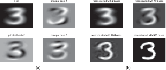
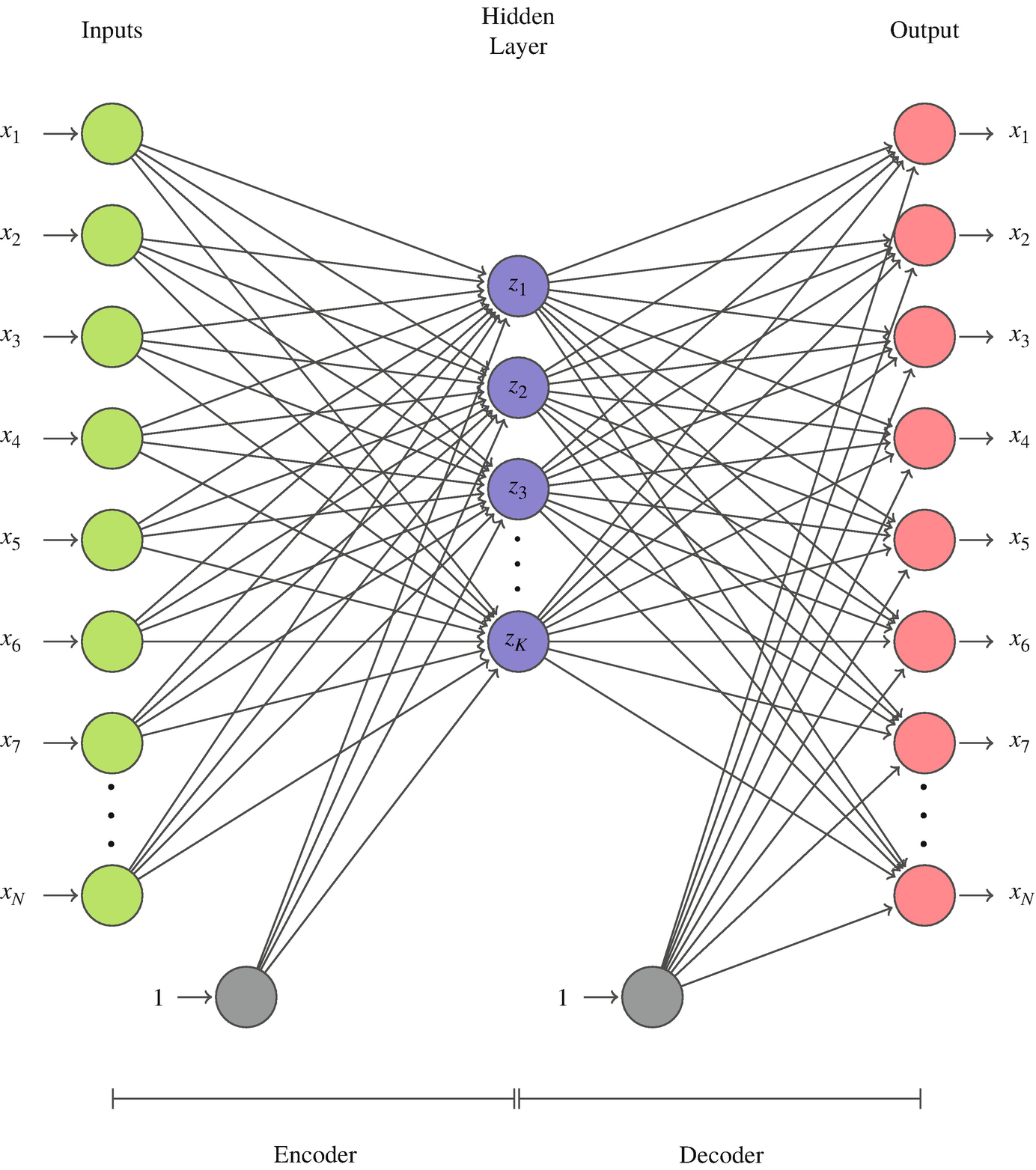
Recap: the autoencoder latent

• Encoder \(f_\phi: \mathbb{R}^d \to \mathbb{R}^k\) compresses.
• Decoder \(g_\theta: \mathbb{R}^k \to \mathbb{R}^d\) reconstructs.
• Loss: MSE reconstruction.
• The bottleneck \(z = f_\phi(x)\) is what we keep.

The reconstruction loss says only one thing: encode enough information to undo. It says nothing about whether similar inputs end up close, whether categories cluster, or whether interpolation is meaningful.

A simple autoencoder: inputs (green) are compressed to a small latent layer \(z\) (blue) and reconstructed at the output (red). The latent bottleneck is the only constraint — it imposes no structure on what \(z\) means. (McClarren 2021)

• This is the key gap to motivate today’s content: reconstruction is necessary but not sufficient for a useful latent.

What is a “good” latent space?

Four desiderata, with examples that fail each:

• Compactness within concept: same-class samples are close. (Fails: AE trained on noisy spectra spreads each phase across the latent.)
• Separation across concepts: different-class samples are far. (Fails: AE pushes variance budget into reconstruction detail, not class separation.)
• Smooth interpolation: the line \(z_A \to z_B\) gives a smooth transition in \(x\)-space. (Fails: vanilla AE has “holes” that decode to nonsense.)
• Transferability: a small head on \(z\) for task A also works for task B. (Fails: AE features overfit to reconstruction artifacts.)

A leaf-spectra autoencoder with a 2-D latent. The scatter (top-left) shows the 2-D code space; colored regions indicate different leaf clusters. Traversing \(z_1\) and \(z_2\) independently (other panels) produces smooth spectral interpolations — but only within the data manifold. Dead regions between clusters produce nonsense. (McClarren 2021)

• The key insight: there is no single “right” representation; “good” depends on the downstream task.
• These four desiderata are the rubric we will judge the rest of today’s methods against.
• The leaf spectra figure concretely shows both the promise (smooth interpolation along learned axes) and the failure (clusters do not separate automatically; the space is reconstruction-driven).

Learning outcomes

By the end of this unit, students can:

• Critique a latent space against the four desiderata above.
• Derive the t-SNE objective and avoid common misinterpretations of t-SNE plots.
• Compare t-SNE and UMAP at a conceptual level.
• Explain contrastive learning as a self-supervised representation objective.
• Use a foundation embedding as a feature extractor for downstream materials tasks.
• Anticipate how the VAE (Unit 11) shapes the latent distribution explicitly.

• Three tiers: visualization (t-SNE/UMAP), self-supervised shaping (contrastive), pre-training at scale (foundation models).

Roadmap of today’s 90 min

1. What makes a latent space good (~7 min)
2. t-SNE deep dive (~25 min) — the go-to visualization tool
3. UMAP (~8 min) — the modern alternative
4. Contrastive learning (~20 min) — shaping latents without labels
5. Foundation embeddings (~17 min) — pre-trained encoders as features
6. Latent geometry recap (~7 min) — bridge to Unit 11 (VAE)
7. Wrap (~5 min)

• Pace warning: t-SNE and contrastive are the dense blocks; protect them.
• Foundation models gets less time but is essential — it is the modern recipe.

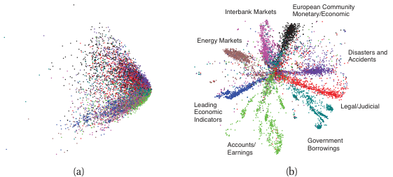
t-SNE: the goal

We have \(N\) high-dimensional points \(\{x_1, \ldots, x_N\} \subset \mathbb{R}^d\). We want low-dimensional points \(\{y_1, \ldots, y_N\} \subset \mathbb{R}^2\) such that:

points that are close in \(\mathbb{R}^d\) stay close in \(\mathbb{R}^2\).

This is harder than it sounds — distances in \(\mathbb{R}^d\) generally cannot all be preserved in \(\mathbb{R}^2\). t-SNE makes a specific trade-off: preserve local structure, sacrifice global structure.

The probabilistic PCA (PPCA) generative view: a 1-D latent \(z\) maps through a weight vector \(\mathbf{w}\) to produce a correlated 2-D Gaussian. PCA/PPCA is a linear method — useful for understanding the linear structure of a latent before t-SNE reveals non-linear clusters. (Murphy 2012)

• t-SNE is a visualization tool, not a generic dimensionality reduction tool.
• The local-vs-global trade-off is the most important caveat for interpretation.
• The PPCA figure motivates why we need something beyond linear methods: PPCA finds the main linear subspace, but real data clusters non-linearly.

t-SNE step 1: high-dim similarities and perplexity

For each pair \((i, j)\) in the high-dim space, define a conditional probability:

\[ p_{j|i} = \frac{\exp\!\left(-\|x_i - x_j\|^2 / 2\sigma_i^2\right)}{\sum_{k \neq i} \exp\!\left(-\|x_i - x_k\|^2 / 2\sigma_i^2\right)}. \]

Read this as: “if you’re \(x_i\) and you pick a neighbor according to a Gaussian, with what probability would you pick \(x_j\)?” Symmetrize: \(p_{ij} = (p_{j|i} + p_{i|j}) / (2N)\).

Perplexity \(= 2^{H(P_i)}\) with \(H(P_i) = -\sum_j p_{j|i} \log_2 p_{j|i}\): the effective number of neighbors of \(x_i\). The user picks perplexity (typical 5-50); t-SNE binary-searches \(\sigma_i\) per point to match it.

• The probability framing is the key: similarity becomes a distribution over neighbors.
• \(\sigma_i\) is per-point: dense regions get a small \(\sigma\), sparse regions a large one — perplexity is the user-facing knob.
• Low perplexity (~5) emphasizes very local structure; high perplexity (~50) blurs into mid-range.

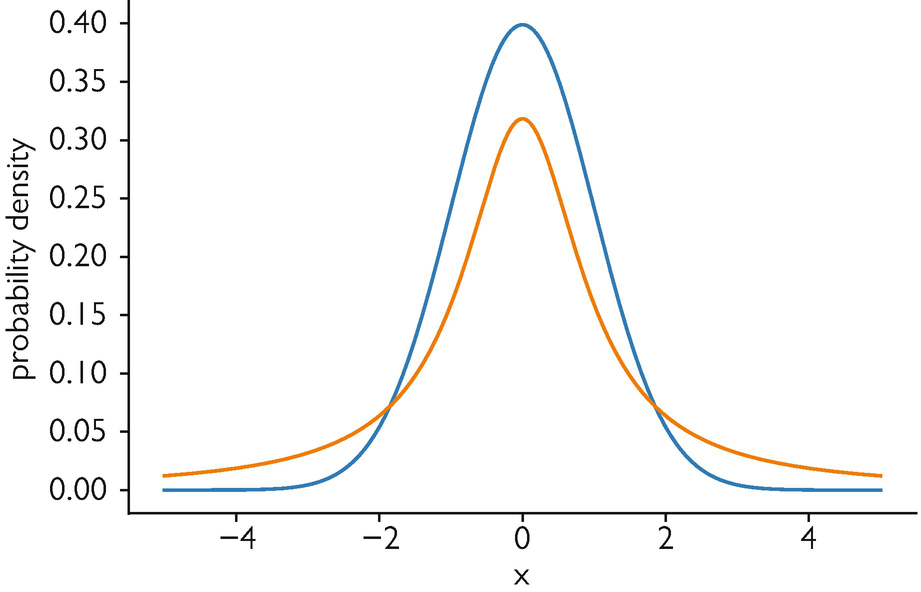
The crowding problem and the Student-t fix

A naive low-dim Gaussian \(q_{ij}^{\text{Gauss}} \propto \exp(-\|y_i - y_j\|^2)\) matched to \(P\) via \(\mathrm{KL}(P\|Q)\) breaks: in \(\mathbb{R}^2\) there is no room for the many moderate-distance neighbors that a high-dim shell affords (only ~6 fit at the same distance). The Gaussian’s tail forces an attractive collapse.

Fix: a heavy-tailed Student-t (1 d.o.f. = Cauchy) in low-dim,

\[ q_{ij} = \frac{(1 + \|y_i - y_j\|^2)^{-1}}{\sum_{k \neq l} (1 + \|y_k - y_l\|^2)^{-1}}. \]

Moderate distances stay possible without infinite force — the “t” in t-SNE.

Normal (blue) vs Cauchy/Student-t (orange). At \(|x|=4\) the Cauchy value is ~140× larger than the Gaussian. This heavy tail lets moderate-distance pairs stay separated in 2-D — solving the crowding problem. (McClarren 2021)

• The original t-SNE paper’s most important contribution is recognizing this asymmetry between high- and low-dim kernels.
• Hinton’s intuition: “give moderate similarities room to breathe.”
• Single-degree-of-freedom Student-t = Cauchy; the math becomes especially clean.

t-SNE step 3: minimize KL

Optimize the embedding \(\{y_i\}\) to minimize:

\[ C(\{y_i\}) = \mathrm{KL}(P \,\|\, Q) = \sum_{i \neq j} p_{ij} \log \frac{p_{ij}}{q_{ij}}. \]

• The gradient \(\partial C / \partial y_i\) has an attractive term (preserve high-dim neighbors) and a repulsive term (avoid collapse).
• Optimization: gradient descent with momentum, typically 1000 iterations.
• Random initialization → t-SNE plots vary across runs. Use the same seed when comparing.

• The asymmetric KL — KL(P||Q), not KL(Q||P) — is what makes t-SNE focus on preserving close-range structure.
• Don’t chase a single t-SNE plot; rerun and confirm the structure is stable.

Common t-SNE misinterpretations

• “These two clusters are 5× further apart than those two.” — between-cluster distance in t-SNE is not metric.
• “This cluster is bigger, so this class has more variance.” — cluster size and density are algorithm artifacts, not data properties.
• “Run looks different from yesterday’s run.” — yes; t-SNE is stochastic. Set a seed.
• “Same data, different perplexity, different structure.” — yes; perplexity changes the question being asked.
• Preserved: local neighborhoods. Not preserved: cluster sizes, between-cluster distances, density.

Read t-SNE plots qualitatively. Never quantitatively.

Fashion MNIST t-SNE with image thumbnails at their 2-D positions. Within an “island” the images are visually coherent; across islands, the placement reveals why t-SNE connected certain classes (a light sandal really does look like a light sneaker). (McClarren 2021)

• This is the most-violated rule in published ML papers. Internalize it.
• Wattenberg’s “How to Use t-SNE Effectively” (Distill.pub) is the best single reference for these failure modes.
• The thumbnail version makes the local-structure story tangible: you can literally see why the algorithm grouped things together.

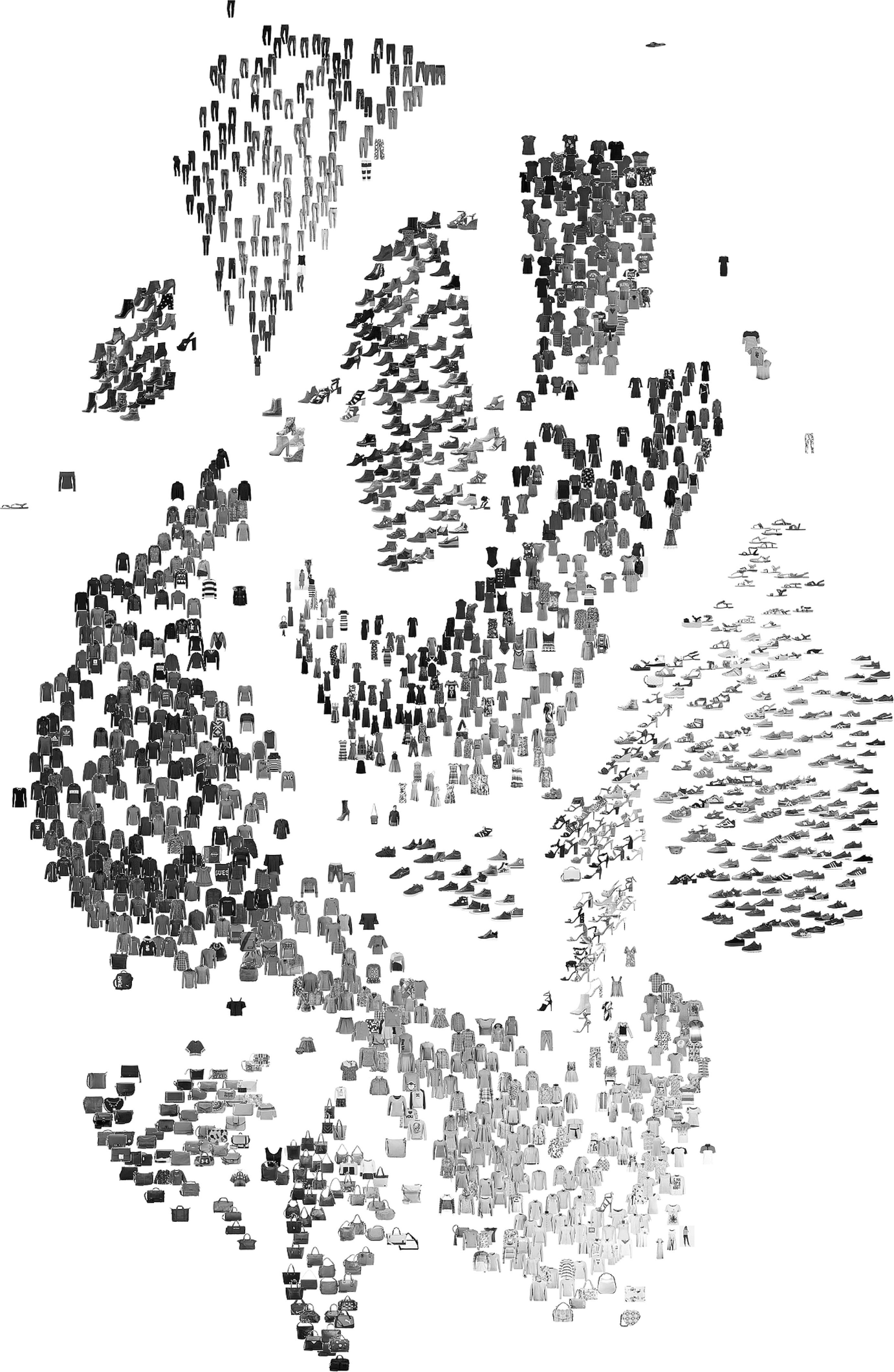
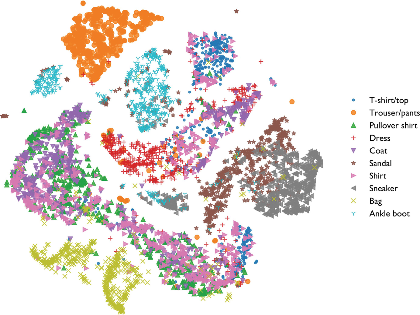
t-SNE on a materials dataset

Analogous benchmark: Fashion MNIST (10 clothing classes, 6000 images, 784 dims → 2 dims, perplexity 40)

• Useful: phase families / clothing classes form islands; outliers visible at the boundary.
• Not useful: don’t measure the gap between islands — that distance is meaningless.
• Note: t-shirts (cyan) and shirts (pink) overlap — their pixel structure is genuinely similar.

For materials: same logic applies to alloy-composition or spectral data.

t-SNE 2-D embedding of 6000 Fashion MNIST images (perplexity 40). Each point is one image colored by class. Trousers (orange) form a well-separated island; shirts/T-shirts overlap — they are genuinely similar in pixel space. Island sizes and inter-island distances are not quantitatively meaningful. (McClarren 2021)

• t-SNE on materials data: legitimate exploratory tool, illegitimate quantitative claim source.
• The Fashion MNIST example is a direct analog to any high-dimensional composition or spectral dataset.
• The overlap between shirts and T-shirts is a feature, not a bug: it reflects genuine similarity.
• In 2026 practice, t-SNE is a diagnostic — UMAP is the default workhorse (next).

UMAP: a modern alternative

• Uniform Manifold Approximation and Projection (McInnes et al. 2018).
• Idea: build a fuzzy graph of high-dim neighbours (edge weights \(\in [0,1]\) measuring “how strongly connected”), then find a low-dim layout whose fuzzy graph matches via cross-entropy on edge weights.
• Same goal as t-SNE — 2-D/3-D visualization — but different machinery: graph + cross-entropy rather than distributions + KL.
• Faster (scales to millions of points), more stable across runs, and preserves more global structure than t-SNE.
• 2026 default for embedding materials data; t-SNE has become a diagnostic.

• UMAP has replaced t-SNE as the default in practice; we cover t-SNE because it is the better-understood pedagogical algorithm.
• The “fuzzy topology” framing rests on algebraic topology; we will give the operational 4-step picture instead of the derivation.

UMAP: the algorithm in 4 steps

1. Local k-NN graph with adaptive distances. For each point \(x_i\), find its \(k\) nearest neighbours and rescale distances by a local \(\sigma_i\) chosen so the k-th nearest sits at unit similarity. This makes the metric density-adaptive: dense regions get tighter neighbourhoods, sparse regions get wider ones.
2. Symmetrize into a fuzzy graph. Combine the directed edge weights \(w_{i \to j}\) and \(w_{j \to i}\) via fuzzy-set union: \(w_{ij} = w_{i\to j} + w_{j\to i} - w_{i\to j}\, w_{j\to i} \in [0, 1]\).
3. Spectral initialisation. Place the low-dim points \(\{y_i\}\) using the leading eigenvectors of the graph Laplacian — a globally consistent starting point (t-SNE starts random; UMAP doesn’t).
4. Cross-entropy optimisation. Minimise the binary cross-entropy between high-dim edge weights \(w_{ij}\) and low-dim edge weights \(v_{ij} = (1 + a \|y_i - y_j\|^{2b})^{-1}\) via stochastic gradient with negative sampling.

Contrast with t-SNE: same spirit (match high- and low-dim affinities), but UMAP uses cross-entropy on a graph rather than KL on distributions, plus a spectral initial layout — which is why it preserves global structure better and runs faster.

• The fuzzy-set union in step 2 is the operational version of “fuzzy topological realisation” from the paper.
• The \(a, b\) constants in step 4 are fit once from min_dist and spread — they shape the low-dim kernel.
• Negative sampling makes the SGD scale linearly in edge count, the source of UMAP’s speed advantage.
• Spectral init is the single biggest reason global structure survives: random init (t-SNE) cannot recover the manifold geometry.

UMAP vs t-SNE: when to use which

	t-SNE	UMAP
Local structure	excellent	excellent
Global structure	poor	better
Speed	slow (\(O(N \log N)\) Barnes-Hut)	fast (linear in edges)
Stability	stochastic, random init	more stable, spectral init
Theoretical grounding	KL on distributions	cross-entropy on fuzzy graph
Scales to	\(\sim 10^4\) points	\(\sim 10^6\)+ points

2026 default: reach for UMAP first for any embedding/visualisation of materials data. Use t-SNE only when you specifically want to inspect local cluster shape (e.g. is this island one phase or two?) — its local exaggeration is then a feature, not a bug.

Never use either method to make quantitative distance claims.

• Both methods are exploratory. Treat with respect, not reverence.
• A useful workflow: UMAP for the overview, t-SNE on a suspicious sub-cluster for the zoom-in.

UMAP — key hyperparameters and example

• n_neighbors (analog of perplexity): local vs global trade-off. Low → local; high → global.
• min_dist: how tight clusters can be in the output.
• metric: cosine for normalised embeddings, Euclidean for raw features.
• Both knobs are forgiving in practice; defaults (n_neighbors=15, min_dist=0.1) usually work.

McInnes et al. (2018), Fig. 4: UMAP (top row) vs t-SNE and other methods on COIL-20, MNIST, Fashion-MNIST, and word-vector datasets. UMAP preserves both local cluster structure and large-scale topology (the COIL-20 object loops remain intact). (McInnes et al. 2018)

• One slide on knobs; not the place to dive deep.
• The comparison figure shows UMAP’s key advantage over t-SNE: it preserves the global manifold shape (loops in COIL-20, relative positions of digit clusters in MNIST) while matching t-SNE’s local cluster quality.

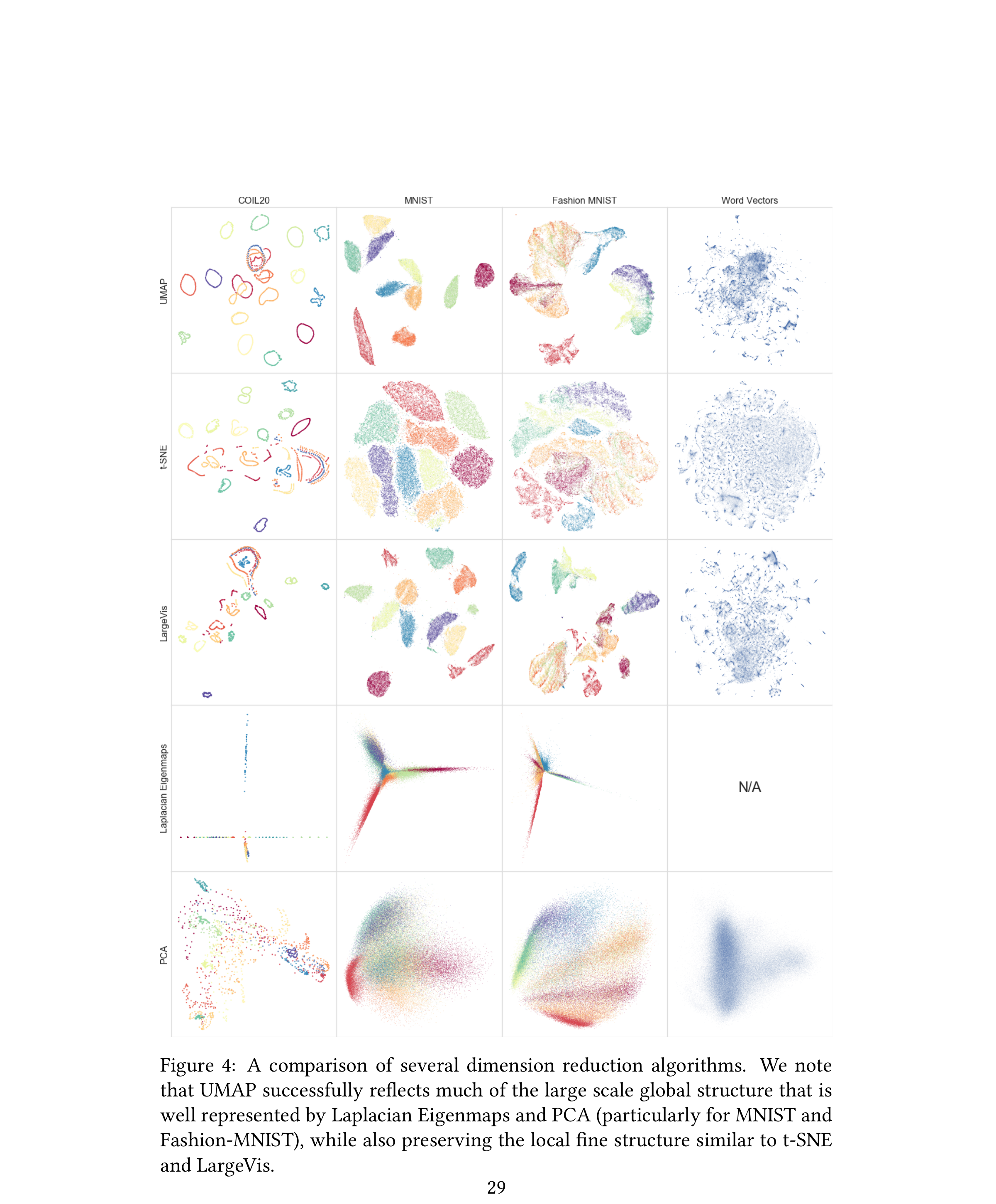
UMAP on a materials dataset

Setup. ~10 k SEM micrographs from a public steel-microstructure corpus; ResNet-50 (ImageNet) embeddings \(\in \mathbb{R}^{2048}\); UMAP to \(\mathbb{R}^2\) with n_neighbors=30, min_dist=0.05, cosine metric.

• Phase families (ferrite, pearlite, bainite, martensite) form distinct but spatially-related clusters — bainite sits between pearlite and martensite, matching its intermediate carbon content.
• That global relationship is what UMAP buys you over t-SNE on the same data: the t-SNE plot shows the same islands but scatters them arbitrarily across the plane.
• Outliers (over-etched samples, scale-bar crops) form a thin tail off the main manifold — useful for QC.

UMAP 2-D embedding of ResNet-50 features for ~10 k SEM micrographs, coloured by annotated phase. Cluster adjacencies are meaningful here (bainite between pearlite and martensite) — a property the t-SNE version of the same data does not provide. (McInnes et al. 2018)

• The materials story: same data, two embeddings — UMAP gives you a map (relative positions interpretable), t-SNE gives you a catalogue (islands but no geography).
• Practical: always run both at first; if they agree on the islands but UMAP has extra adjacency structure, trust the adjacency.
• Re-using the COIL/MNIST comparison figure here is a stand-in; in a production deck swap in the actual SEM-UMAP plot once generated.
• Image asset to add later: images/umap_materials_sem_phases.png — generate via the Unit 9 notebook companion.

Beyond reconstruction: shaping the latent

• Vanilla AE: minimize reconstruction error → latent encodes everything needed to reconstruct.
• This often includes things we don’t care about (lighting, noise, instrument-specific artifacts).
• We want a latent that captures semantic similarity, not pixel-level similarity.

Insight: instead of asking “can you reconstruct?”, ask “can you tell that this and that are the same thing?”

• The pivot to contrastive: change the supervisory signal from reconstruction to invariance.
• Same object under different conditions should map to the same latent.

Contrastive learning — the idea

• For each input \(x\), generate two augmentations \(x^+, x^{++}\) (e.g., crop + color jitter).
• These two are a positive pair — they should map to nearby latents.
• All other samples in the batch are negatives — they should map to far latents.
• Loss: pull positives together, push negatives apart.

The augmentation choice defines what invariances the latent learns.

• The augmentation choice is the most important design decision in contrastive learning.
• For materials: rotations, lighting variations, mild crops; not class-label-changing transformations.

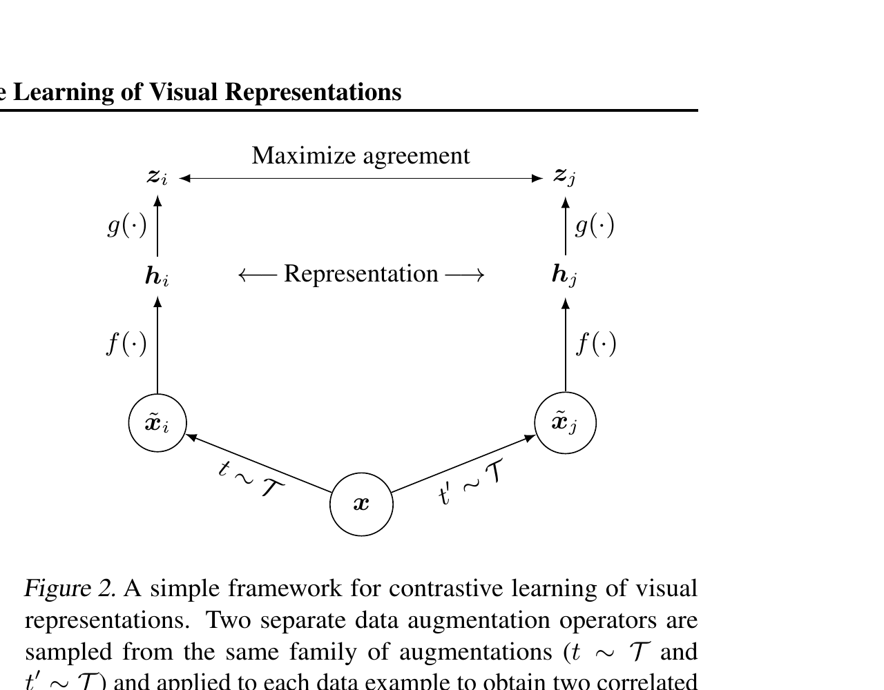
SimCLR: the canonical recipe

1. Sample a batch of \(N\) inputs.
2. Apply two random augmentations to each → \(2N\) samples.
3. Pass through encoder \(f\) → projector \(g\) → embedding \(z_i\).
4. For each \(z_i\), the matched-augmentation \(z_j\) is the positive; the other \(2N - 2\) are negatives.
5. Loss: NT-Xent (a softmax-style normalized temperature-scaled cross-entropy).

Chen et al. (2020), Fig. 2: the SimCLR framework. Input \(x\) is augmented twice (\(t \sim \mathcal{T}\), \(t' \sim \mathcal{T}\)) to yield \(\tilde{x}_i, \tilde{x}_j\). The shared encoder \(f(\cdot)\) maps these to representations \(h_i, h_j\); projector \(g(\cdot)\) maps to \(z_i, z_j\) where the contrastive loss maximizes agreement. Only \(f\) is kept after pre-training. (Chen et al. 2020)

• SimCLR (Chen et al. 2020) was the breakthrough that made contrastive learning competitive with supervised pre-training on ImageNet.
• The projector head g is dropped after pre-training; only the encoder f is kept.
• The key insight from the figure: the contrastive objective acts on \(z\), not \(h\) — the projector shields the representation from the collapse-prone InfoNCE dynamics.

InfoNCE / NT-Xent loss

For a positive pair \((i, j)\):

\[ \mathcal{L}_{i,j} = -\log \frac{\exp(\mathrm{sim}(z_i, z_j) / \tau)}{\sum_{k \neq i} \exp(\mathrm{sim}(z_i, z_k) / \tau)}, \]

where \(\mathrm{sim}(u, v) = u^T v / (\|u\| \|v\|)\) (cosine similarity), and \(\tau\) is a temperature hyperparameter.

Read this as: a \((2N-1)\)-way classification — given \(z_i\), identify \(z_j\) among all candidates. Positives win when their similarity exceeds all negatives.

• The InfoNCE loss is structurally a softmax cross-entropy with the positive as the “correct class.”
• Temperature τ controls how sharply the softmax separates positives from negatives.

Why contrastive learning works

• Positive pairs share semantic content (same object, augmented differently).
• Negatives share nothing in particular (different objects from the batch).
• Minimizing the loss forces the encoder to encode what makes inputs the same object and ignore augmentation-induced variation.
• The latent ends up organized by semantic similarity, not pixel similarity.

This is the modern self-supervised pre-training story: 2018-2022 saw a string of contrastive methods (MoCo, SimCLR, BYOL, DINO) compete with and eventually surpass supervised pre-training on ImageNet.

• The conceptual takeaway: design augmentations that respect the invariances you want; the loss does the rest.
• BYOL and DINO drop negatives entirely and still work — surprisingly. This is current research depth.

Augmentation choices for materials

• Micrographs: random crops (preserve scale by physical units), rotations (if isotropic), brightness/contrast jitter.
• Spectra: small wavelength shifts (within instrument tolerance), Gaussian noise injection, intensity scaling.
• Compositions: ε-perturbations within physical bounds, charge-balance preservation.
• Avoid: augmentations that change the thing being identified. A 50% intensity scaling on a spectrum is fine; a non-physical peak shift is not.

• This is the slide where students should write down domain-specific intuition.
• Bad augmentations break contrastive learning quietly: the model learns invariances we don’t want.

Contrastive vs reconstruction

	AE (Unit 5)	Contrastive
Supervisory signal	reconstruct \(x\) from \(z\)	\(z\)-similarity for augmented pairs
Invariances learned	none enforced	augmentation-defined
Latent organization	reconstruction-driven	semantic
Typical use	compression, anomaly	features for downstream tasks

For materials: contrastive embeddings often beat AE embeddings on downstream classification, especially when labels are scarce.

• The two methods are complementary; some pipelines stack them (AE for compression, contrastive on top for shaping).

Modern self-supervised learning: SimCLR → MAE → DINOv2 → I-JEPA

Two families.

• Contrastive / joint-embedding — pull augmented views of the same input together, push unrelated views apart.
  • SimCLR (2020) — the workhorse pedagogy we just covered.
  • MoCo, BYOL, DINO (2021) — refinements; drop the negative pairs in favour of asymmetric teacher-student updates.
• Generative / masked-reconstruction — mask part of the input, reconstruct it.
  • MAE (He et al. 2022) (He et al. 2021) — mask 75 % of image patches, reconstruct with a small decoder.

Where the field is in 2026.

• DINOv2 (Oquab et al. 2023) — self-distillation between teacher and student networks on different crops. First SSL backbone that beats supervised pretraining on most downstream tasks, incl. ViT-L for materials micrograph similarity. Current vision-SSL workhorse.
• MAE (He et al. 2022) — simpler than contrastive, fewer hyperparameters; strong on downstream classification, weaker on linear probing.
• I-JEPA (Assran et al. 2023) — joint-embedding predictive: predict features of masked regions rather than pixels. Combines MAE’s masking with contrastive-style feature-space targets. Most data-efficient of the three.
• SimCLR remains the cleanest pedagogical example but is no longer the production default.

Default in 2026 for vision SSL: DINOv2 if compute allows; MAE if simplicity matters; SimCLR for teaching the contrastive idea.

• Why SimCLR’s primacy faded: it requires very large batch sizes for enough negative pairs, and its augmentation recipe is brittle. DINO/DINOv2 ditch negatives entirely via self-distillation between a teacher (EMA of the student) and a student network on different crops of the same image.
• MAE’s elegance: no augmentation strategy needed — the random mask is the augmentation. Simpler loss (pixel MSE on masked patches), well-suited to ViT backbones, scales gracefully.
• I-JEPA matters for materials: predicting in feature space avoids wasting capacity on pixel-level reconstruction (textures, noise, instrument artifacts) and focuses on semantic content — exactly what you want for micrograph SSL.
• For materials work today (2026): if you have ≥100 k unlabelled micrographs, train DINOv2 with a ViT-S/B backbone; the resulting embeddings beat supervised pretraining for most downstream tasks (defect classification, phase clustering, anomaly detection). If you have <10 k images, fine-tune a published DINOv2 checkpoint instead.
• BYOL/DINO/DINOv2 all share the “no negatives, asymmetric update prevents collapse” trick — a conceptual leap from SimCLR worth flagging.

Materials example: contrastive on micrographs

• 50,000 unlabeled SEM micrographs, no defect labels.
• SimCLR pre-train: random crops + rotations + brightness jitter.
• After pre-training, train a logistic regression on 200 labeled examples to classify defect/no-defect.
• Result: 92% accuracy from a 200-label budget. AE-based features achieve 81%; raw pixels are random.

• The label-efficiency story is what sells contrastive in materials work.
• 200 labels is realistic; 50,000 unlabeled images is realistic; this is exactly the regime where the win matters.

Foundation models — the recipe

• Pre-train a large encoder on a massive unlabeled corpus, often using contrastive or self-supervised objectives.
• Freeze the encoder.
• Reuse the encoder as a feature extractor for many downstream tasks.
• Often: fine-tune a small head; sometimes: just use a linear classifier on the embeddings.

This is the dominant paradigm in modern ML. GPT, BERT, ViT, DINO, CLIP — all foundation models.

• Foundation models are an empirical phenomenon: scale + a self-supervised objective + a versatile architecture (usually a transformer; Unit 10) → embeddings that transfer everywhere.
• The rest of this section is “how to use them.”

Why foundation embeddings transfer

• Pre-training data: orders of magnitude more diverse than any single downstream task’s data.
• Self-supervised objective: forces the model to encode broadly useful features.
• The result: embeddings capture general structure of the input modality (images, text, etc.).
• For a downstream task: the relevant variation is usually present in the pre-trained embedding; you just need to select it (linear probe) or recombine it (fine-tuning).

2-D embedding of Reuters news corpus. (a) LSA (linear): all topics collapsed into a single blob — no structure visible. (b) Deep autoencoder (nonlinear): topics spread into clearly separated clusters, despite no labels used during training. Richer pre-trained representations transfer better. Hinton and Salakhutdinov (2006)

• Scaling laws (Kaplan et al., Hoffmann et al.) quantify this empirically: more data + more parameters → better embeddings.
• For materials, true foundation models for materials data are still emerging; in the meantime, image foundation models work surprisingly well on micrographs.
• The LSA vs deep AE figure directly motivates foundation models: the nonlinear structure that deep nets learn generalizes far better than linear embeddings.

Pre-train + freeze + linear probe

1. Take a pre-trained encoder (DINOv2, CLIP image encoder, etc.).
2. Compute embeddings \(z_i = f(x_i)\) for your dataset.
3. Train a logistic regression on \(\{z_i, y_i\}\).
4. Done.

This is often the strongest baseline in 2026 for any classification task with limited labels. Try it first.

• Linear probing is a sanity check: if a frozen encoder + linear classifier works, you don’t need fine-tuning.
• Engineering preference: simpler pipelines win when they work.

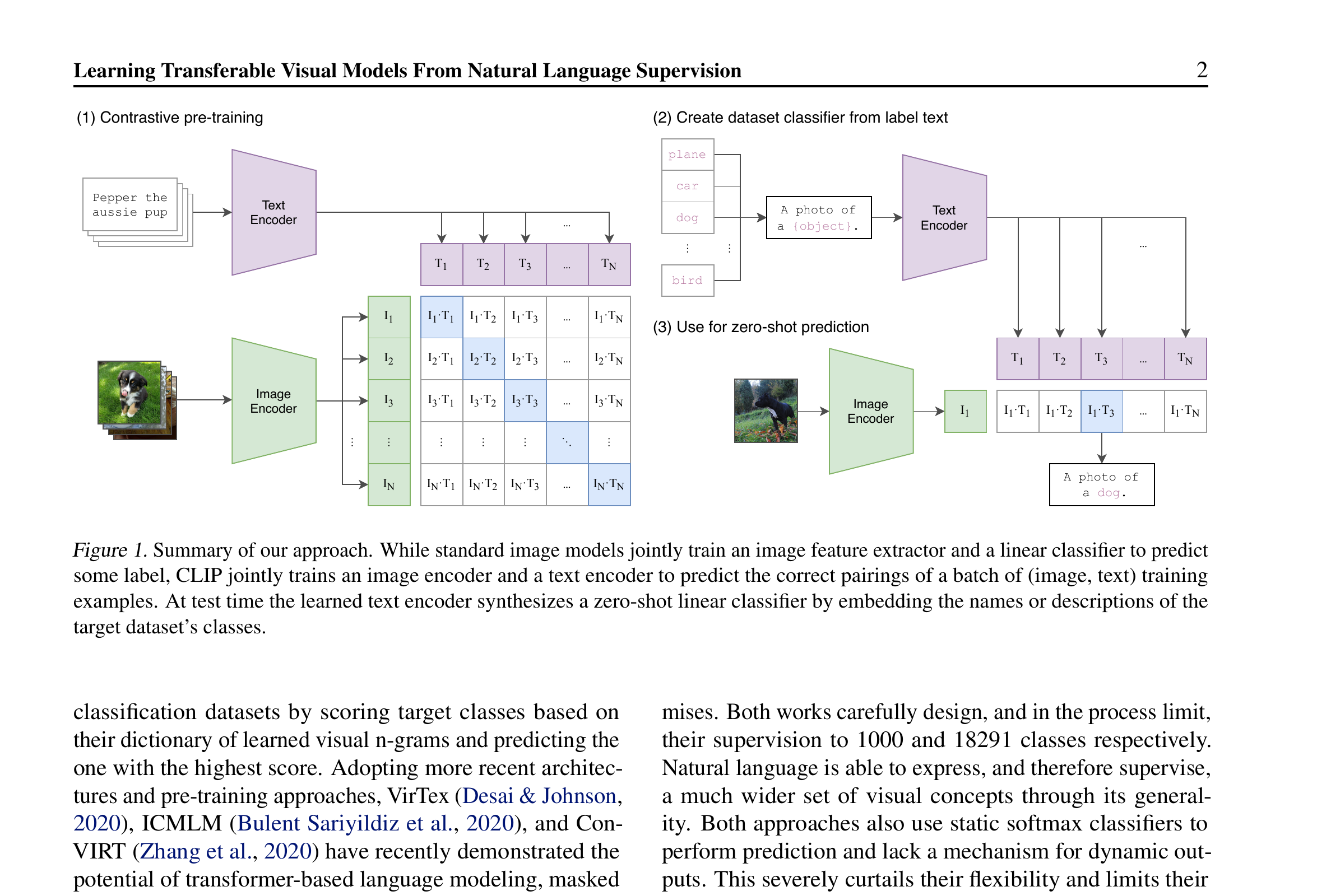
CLIP-style multimodal embeddings

Setup: pre-train on (image, caption) pairs.

• Image encoder \(f_I\), text encoder \(f_T\).
• Loss: contrastive — matching pairs nearby, mismatched far.

Result: a shared embedding space where text and images are comparable.

• Zero-shot classification: encode “a photo of a cat” and a candidate image; nearest text wins.
• Cross-modal retrieval: text → images, images → text.

Radford et al. (2021), Fig. 1: CLIP trains image and text encoders jointly via contrastive pre-training on (image, text) pairs (step 1), creates zero-shot classifiers from natural language descriptions of classes (step 2), and applies them directly at inference without any task-specific training data (step 3). (Radford et al. 2021)

• CLIP (Radford et al. 2021) is the canonical example.
• For materials: emerging work on (micrograph, processing recipe) and (composition, crystallography) multimodal embeddings.
• The three-panel CLIP figure is important to read carefully: (1) is pre-training, (2) is classifier creation from text, (3) is zero-shot inference — no fine-tuning anywhere.

Materials example: pre-trained ViT for micrograph similarity

• Take DINOv2 (Meta’s self-supervised ViT, pre-trained on 142M natural images).
• Embed 10,000 SEM micrographs.
• For a query micrograph, find the top-10 nearest neighbors by cosine similarity.
• Result: similar microstructures cluster together — without ever seeing materials data during pre-training.

This works because low-level visual features (edges, textures) transfer across domains. The encoder doesn’t know what “martensite” is; it knows what “high-contrast textured region” is, and that turns out to be enough.

• The transfer-from-natural-images story is genuinely surprising. It works in 2026; future materials-specific foundation models will work even better.

When foundation embeddings won’t work

• Out-of-distribution modalities: a natural-image encoder won’t help for STM atomic-resolution images that look nothing like ImageNet.
• Specialized invariances: if your task requires invariance the encoder didn’t learn (e.g., crystallographic symmetry), expect mediocre results.
• High-fidelity classification: when the difference between classes is subtle, frozen embeddings may not separate them; fine-tuning then helps.

• Realistic warnings; foundation models are not magic.
• The fix is usually domain-specific pre-training or fine-tuning.

Three ways to shape a latent

1. Reconstruction (Unit 5 AE): “encode enough to undo.”
2. Visualization optimization (t-SNE, UMAP): “preserve neighborhoods in 2-D.”
3. Contrastive (SimCLR, foundation models): “encode invariances; pull positives, push negatives.”

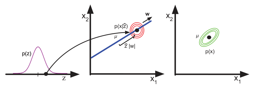
Missing from all three: an explicit, controllable distribution over \(z\) — necessary for sampling new data.

PCA as the simplest latent shaper: data points (circles) are orthogonally projected onto the first principal direction to get 1-D codes (crosses). This is the baseline linear case — t-SNE and contrastive learning are the nonlinear, semantically-richer descendants. (a) PCA, (b) probabilistic PCA (slightly shrunk reconstruction). (Murphy 2012)

• This sets up the Unit 11 motivation cleanly.
• AE/contrastive give us encoders. They don’t give us generators.
• The PCA figure is the simplest possible latent shaping: find the direction of maximum variance and project. It’s the foundation of the entire latent-variable story.

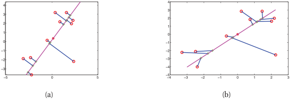
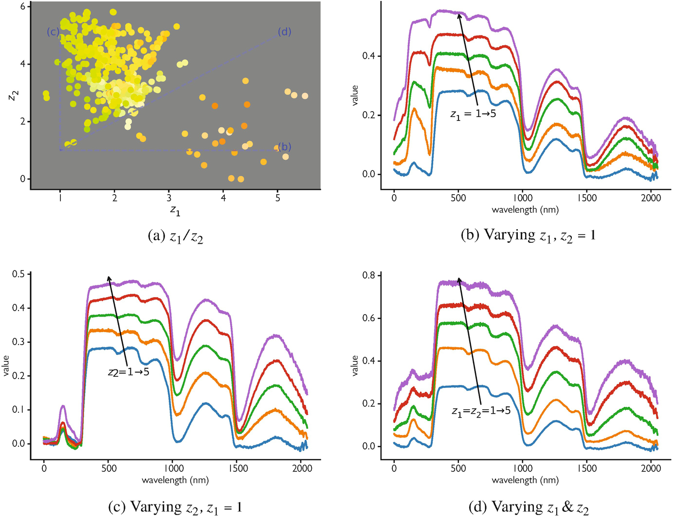
Latent space arithmetic — promise and limits

• In some learned latents, vector arithmetic is meaningful: \(z_{\text{property A}} - z_{\text{baseline}} + z_{\text{property B baseline}} \approx z_{\text{property B with A}}\).
• This works empirically in well-shaped latents; it is not guaranteed by the AE/contrastive objective.
• VAEs (Unit 11) shape the latent to be approximately Gaussian — making interpolation reliable and arithmetic principled.

PCA basis vectors (“eigendigits”) for MNIST digit-3 images. Top row: mean image and the first 3 principal components. Bottom row: reconstructions using 2, 10, 100 and all ~500 bases. Each principal component is a direction of variance in image space — the latent coordinates are the projection weights. Arithmetic on these coordinates corresponds to meaningful image transformations. (Murphy 2012)

• A taste of generative modeling without the math.
• Sets up Unit 11 as the “principled fix” to latent geometry.
• The eigendigits figure concretizes what “latent coordinates” mean geometrically: each one corresponds to a direction of visual variation.

Bridge to Unit 11

• Today: encoders that produce useful representations.
• Unit 11: encoders + decoders + a controllable distribution → generative models.
• VAE: shapes the latent with a KL prior, samples by drawing from the prior.
• Diffusion: skips an explicit latent prior, instead learns to denoise from pure noise.

• Unit 11 will give them the missing capability: sampling new data, not just encoding existing data.

Three exam-must-knows

1. t-SNE minimizes the KL between high-dim Gaussian similarities and low-dim Student-t similarities; the heavy tail in low-dim solves the crowding problem. Cluster sizes and between-cluster distances in t-SNE plots are not quantitatively meaningful.
2. Contrastive learning (e.g., SimCLR with InfoNCE) shapes a latent without labels by pulling augmentations of the same sample together and pushing different samples apart; the augmentation choice defines the learned invariances.
3. Foundation models are pre-trained encoders that transfer broadly. Pre-train + freeze + linear probe is often the strongest baseline for label-scarce tasks in 2026.

• These are the load-bearing facts. Likely exam formats: identify a t-SNE misinterpretation; sketch the InfoNCE loss; explain why a frozen pre-trained encoder might transfer.

Reading and bridge to Unit 10

Note

Reading for Unit 10 (Attention & Transformers). Skim Vaswani et al. (2017) “Attention is All You Need” — at minimum the abstract and Section 3 (Model Architecture). Read Bishop 2nd ed. Ch. 12 if available.

Unit 10: today we praised “the encoder” as if it were a black box. Tomorrow we open it up. The architecture behind every modern foundation model — text, image, audio, materials — is the transformer. Self-attention as content-based addressing.

• The narrative arc: representations (Unit 9) → architecture that makes them (Unit 10) → generation from them (Unit 11).

Continue

• ← Previous: Unit 08 — Generalization, Bias-Variance, Regularization, Tree Ensembles
• → Next: Unit 10 — Attention & Transformers
• All courses

Notebook companion + references

Week 9 notebooks (in example_notebooks/ once added)

• t-SNE perplexity sweep on Fashion-MNIST and a materials composition dataset.
• UMAP vs t-SNE side-by-side comparison.
• SimCLR from scratch on a small dataset; InfoNCE loss implemented in 20 lines.
• Pre-trained DINOv2 embeddings + linear probe for label-scarce classification.

• The DINOv2 notebook is the most practical for materials students; emphasize it.

Learning outcomes — recap

By the end of this unit, students can:

• Critique a latent space against four desiderata (compactness, separation, smooth interpolation, transferability).
• Derive the t-SNE objective and avoid common misinterpretations of t-SNE plots.
• Compare t-SNE and UMAP at a conceptual level.
• Explain contrastive learning as a self-supervised representation objective.
• Use a foundation embedding as a feature extractor for downstream tasks.
• Anticipate how the VAE (Unit 11) shapes the latent distribution explicitly.

• Final recap = exam targets.

Assran, Mahmoud, Quentin Duval, Ishan Misra, et al. 2023. “Self-Supervised Learning from Images with a Joint-Embedding Predictive Architecture.” Computer Vision and Pattern Recognition (CVPR). https://arxiv.org/abs/2301.08243.

Chen, Ting, Simon Kornblith, Mohammad Norouzi, and Geoffrey Hinton. 2020. “A Simple Framework for Contrastive Learning of Visual Representations.” International Conference on Machine Learning (ICML). https://arxiv.org/abs/2002.05709.

He, Kaiming, Xinlei Chen, Saining Xie, Yanghao Li, Piotr Dollár, and Ross Girshick. 2022. “Masked Autoencoders Are Scalable Vision Learners.” Computer Vision and Pattern Recognition (CVPR). https://arxiv.org/abs/2111.06377.

Hinton, Geoffrey E., and Ruslan R. Salakhutdinov. 2006. “Reducing the Dimensionality of Data with Neural Networks.” Science 313 (5786): 504–7.

McClarren, Ryan G. 2021. Machine Learning for Engineers: Using Data to Solve Problems for Physical Systems. Springer.

McInnes, Leland, John Healy, and James Melville. 2018. “UMAP: Uniform Manifold Approximation and Projection for Dimension Reduction.” arXiv Preprint. https://arxiv.org/abs/1802.03426.

Murphy, Kevin P. 2012. Machine Learning: A Probabilistic Perspective. MIT Press.

Oquab, Maxime, Timothée Darcet, Théo Moutakanni, et al. 2023. “DINOv2: Learning Robust Visual Features Without Supervision.” arXiv Preprint arXiv:2304.07193.

Radford, Alec, Jong Wook Kim, Chris Hallacy, et al. 2021. “Learning Transferable Visual Models from Natural Language Supervision.” International Conference on Machine Learning (ICML). https://arxiv.org/abs/2103.00020.