Mathematical Foundations of AI & ML
Unit 8: Tree Ensembles for Tabular Learning

Prof. Dr. Philipp Pelz

FAU Erlangen-Nürnberg

Title + Unit 8 positioning

• Units 6–7 already gave us the conceptual machinery: loss landscapes, the bias–variance trade-off, regularization, and the probabilistic view.
• This unit cashes that in on the single most important model family for tabular data: decision trees and their ensembles.
• Random forests and gradient boosting are the workhorses of applied materials ML — and the prerequisite for ML-PC Units 7–8 and Materials Genomics.
• The whole unit is one sentence of bias–variance theory turned into two algorithms: bagging reduces variance, boosting reduces bias.

• Set the framing explicitly and honestly: the generalization / bias–variance / regularization theory was developed in Units 6–7, so we do not re-derive it here. This unit is the applied payoff — the models a working materials engineer actually reaches for.
• The stakes for this cohort: on tabular materials data (compositions + processing parameters + measurements), gradient-boosted trees beat neural networks the large majority of the time. If a student leaves this course able to use exactly one model well, it should be a gradient-boosted tree — CatBoost for the categorical-heavy materials data they’ll actually face — say that out loud.
• The unifying thesis, repeated all lecture: every method here is a move along the bias–variance trade-off. Keep “bagging ↓variance, boosting ↓bias” on the board the entire 90 minutes.
• Timing: ~5 min framing, ~25 min trees, ~25 min bagging/RF, ~25 min boosting/GBM, ~10 min practice/comparison/materials. The three interactives are the pace buffers.

Learning outcomes for Unit 8

By the end of this lecture, students can:

• explain how a decision tree partitions feature space and how splits are chosen by impurity reduction,
• state why a single deep tree is a low-bias / high-variance learner,
• derive why bagging reduces variance and why the tree-correlation \(\rho\) caps that reduction,
• explain random forests as bagging + feature subsampling, and read OOB error and feature importances correctly,
• describe gradient boosting as gradient descent in function space, and the role of shrinkage and early stopping,
• choose appropriately between random forests, gradient boosting, and neural networks for a given tabular problem.

• Use the list as a contract, not a recitation. Each bullet is one block of the lecture and maps to the exam slide at the end.
• Flag the two outcomes students most underestimate: (1) the correlation ceiling — why RF exists and not just bagging; (2) reading feature importance correctly — impurity importance is biased and routinely over-interpreted in materials papers. These two are the “you’ll use this in your thesis next month” items.
• Rigor level: derivations to the point of insight (the bagging variance formula, functional-gradient view), not measure-theoretic completeness. Engineering foundations course.

Bias–variance in one slide (the only theory we need)

\[\mathbb{E}[(y-\hat f(x))^2] = \underbrace{\mathrm{Bias}[\hat f]^2}_{\text{too rigid}} + \underbrace{\mathrm{Var}[\hat f]}_{\text{too sensitive}} + \underbrace{\sigma^2}_{\text{irreducible}}\]

• Bias: error from a model class too simple to capture the truth.
• Variance: error from sensitivity to the particular training sample.
• Irreducible \(\sigma^2\): aleatory noise — no model removes it (Unit 7).

• A single deep tree: low bias, high variance.
• Bagging / Random Forest: average many high-variance trees → drive variance down.
• Boosting: sequentially correct a biased ensemble → drive bias down.
• Everything in this unit is one of these two moves.

• This is the only recap — deliberately one slide. Units 6–7 derived it; here it is purely the lens through which every algorithm is read. Do not re-derive; if students want the derivation, point back to Unit 8’s predecessor material / Bishop §3.2.
• Write the two-arrow summary on the chalkboard and leave it: “bagging → ↓Var, boosting → ↓Bias.” Every subsequent slide should be relatable to one arrow. When you introduce RF, point at the Var arrow; when you introduce GBM, point at the Bias arrow.
• Pre-empt the common confusion: bagging does not reduce bias (the trees are already low-bias), and boosting does not primarily reduce variance (it can even increase it — hence early stopping). Saying this now prevents the most frequent exam mistake.

First, the intuition: name that tree

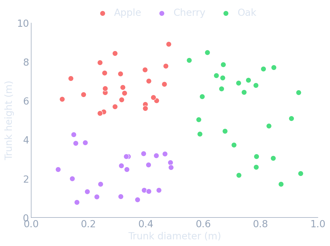
You are a farmer with a new plot of land. For each tree you can measure only two things — the trunk’s diameter and its height — and you must decide: Apple, Cherry, or Oak?

• No equations yet. Just look at the scatter and ask: where would you draw lines to separate the colours?
• This is the whole idea of a decision tree: split the space with simple questions until each region is (almost) one kind of tree.

Three species in (diameter, height) space. The pattern is obvious to the eye — our job is to make a machine find it.

• Deliberately concrete and example-first — this cohort has never seen a decision tree, so we build the picture before any impurity formula. Borrowed pedagogy from the MLU-explain “Decision Trees” explainer (mlu-explain.github.io/decision-tree).
• Ask the room to literally point at where they’d cut. Almost everyone says “diameter splits Oak off first” — that is exactly what the algorithm will discover two slides later. Let them predict it.
• Two features only so the partition is drawable on the board; emphasise that the real materials version has dozens of features and the same logic applies.

Carve the space with yes/no questions

Two axis-aligned cuts split the plot into three pure-ish regions.

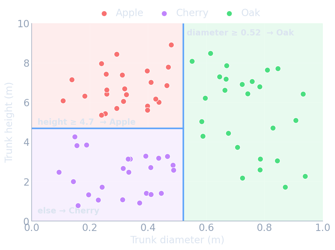
• First cut: diameter ≥ 0.52? → everything to the right is Oak.
• Second cut (left part only): height ≥ 4.7? → tall ones are Apple, short ones are Cherry.
• Each cut is a vertical or horizontal line — a question about one feature at a time.
• A new tree? Measure it, see which box it lands in, predict that box’s majority species.

• The key visual: cuts are axis-aligned (perpendicular to one axis). This is the seed of “axis-aligned splits / hyper-rectangles” on the formal slide that follows — point forward to it.
• Stress recursive: the second question is asked only inside the left region. Nesting questions = the tree structure on the next slide, and = “interactions for free” later.

…and that is literally a decision tree

The same two cuts, drawn as a flowchart: internal nodes ask questions, leaves give answers.

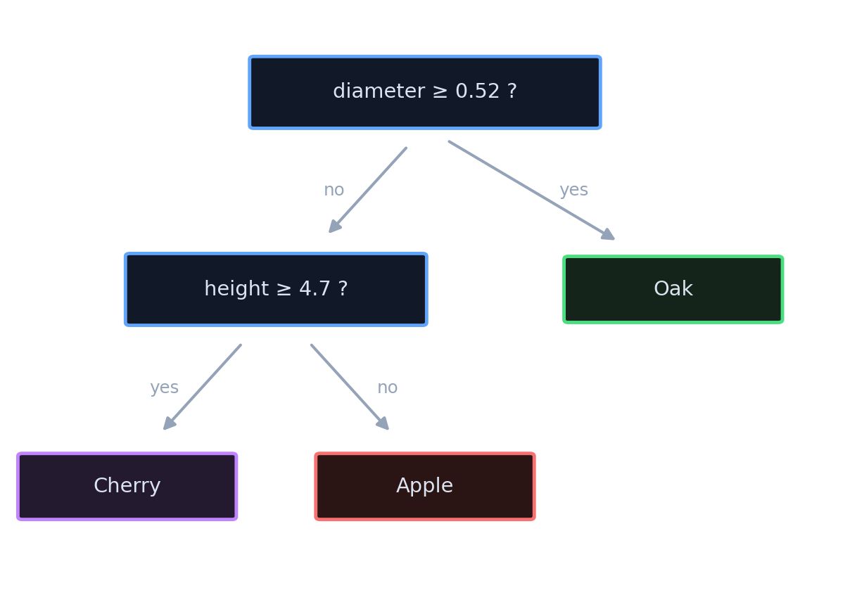
• Boxes on the previous slide ⇔ leaves here. Same model, two pictures.
• Internal node = a yes/no question on one feature.
• Leaf = a prediction (the majority class of the points that reach it).
• To classify a new tree, start at the top and follow the yes/no arrows down to a leaf.

• Make the equivalence explicit by tracing one point through both pictures: pick a small-diameter, tall tree → right partition cell and left-then-Apple path. Same answer.
• This is the payoff slide of the intuition block: students now own the object before we formalise it. Everything after (impurity, greedy search, ensembles) is “how do we build this automatically and reliably.”

Which question is best? Measure “purity”

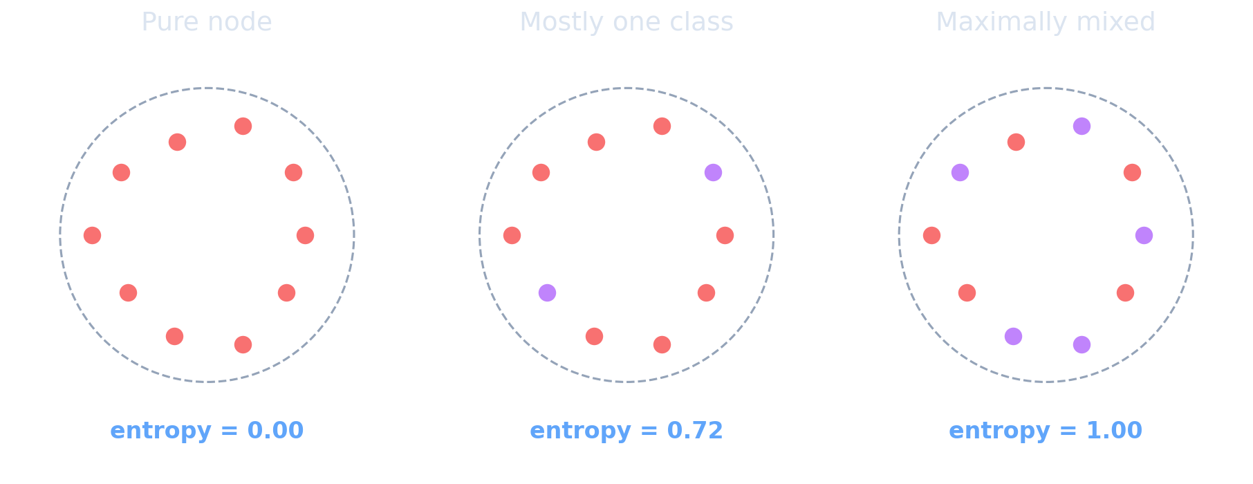
A node is pure if it holds one class, impure if it is a mix. Entropy (also Gini) puts a number on it: 0 = pure, larger = more mixed.

• A good question makes the resulting regions more pure than the parent.
• We will measure impurity with entropy \(-\sum_c p_c \log p_c\) or Gini \(\sum_c p_c(1-p_c)\) — formalised in a moment.

• Entropy intuition only here — the formula is on the upcoming impurity slide, so this is a soft landing, not a derivation. “Pure = boring = zero information left to gain.”
• Connect to the next slide: if we can score purity, we can score a split by how much purity it buys → information gain.

Pick the split with the biggest payoff

Sweep the diameter threshold; the information gain (drop in impurity) peaks at the best cut — exactly the line we drew by eye.

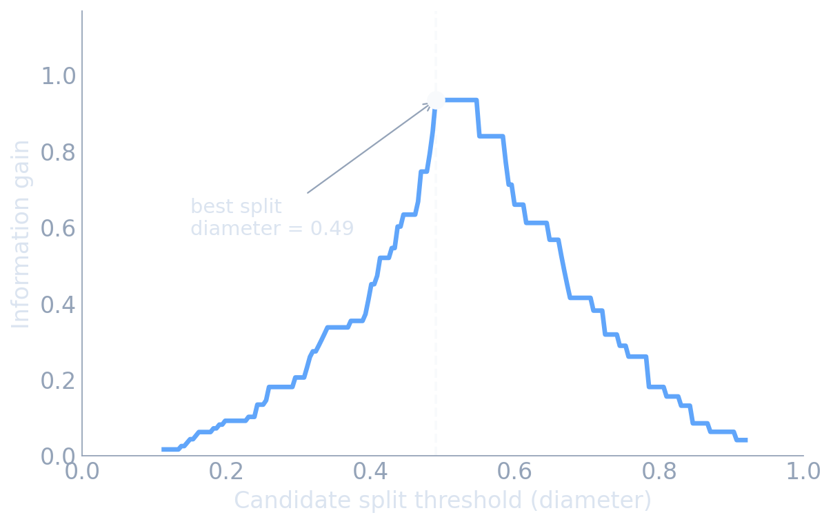
• Try every feature and every threshold; score each by the impurity it removes.
• Keep the single best split, then recurse on each child region.
• Greedy: best question now, no looking back — fast, but not globally optimal.
• The eye-balled “diameter ≈ 0.5” cut is the algorithm’s peak. The intuition was the math.

• This is the bridge to the formal “How splits are chosen” slide: \(\Delta = I(\text{parent}) - \frac{N_L}{N}I(\text{left}) - \frac{N_R}{N}I(\text{right})\) is precisely the curve’s height.
• Greedy + recursive is the entire training algorithm. Say it plainly: no gradient descent, no global objective — just repeat “best cut, then split.”

One tree is powerful — but fragile

Nudge just 10 % of the points (circled) and a fully grown tree redraws its boxes completely.

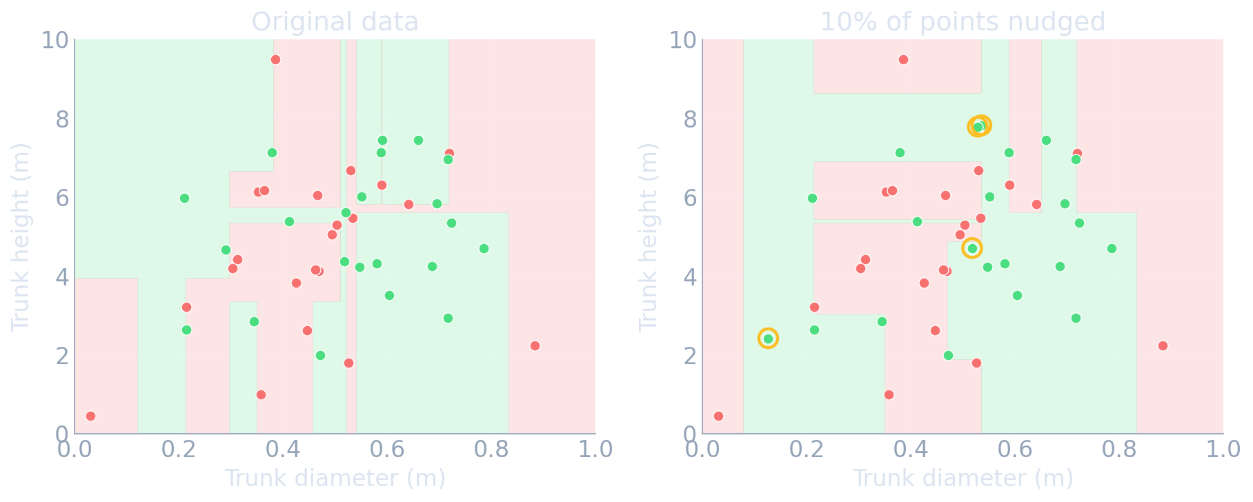
• A single deep tree can fit anything — including the noise (high variance).
• Small data changes → very different tree → the variance arrow on the board.
• The fix, the rest of this unit: average many trees (bagging / forests) and stack corrective trees (boosting).
• Hold onto this picture — it is why ensembles exist.

• This closes the intuition arc and re-points at the bias–variance summary still on the chalkboard: a single tree sits at the high-variance end. Bagging/RF pulls variance down; boosting pulls bias down.
• Honest framing: trees are not weak — they are unstable. Ensembles trade a little interpretability for a lot of stability. That trade is the spine of §2–§3.
• Instability illustration follows MLU-explain’s “problem of perturbations” section — same lesson, our orchard data.

Decision trees — a single learner

A decision tree recursively partitions input space by axis-aligned splits.

• Internal node: a test like “Cr fraction \(> 0.18\)?”
• Leaf: a constant prediction — mean of the leaf’s targets (regression) or majority / class frequencies (classification).
• Prediction: route a new \(x\) down the tree to its leaf and return that constant.

• Non-parametric: model capacity grows with depth, not a fixed parameter count.
• Handles mixed feature types (continuous, ordinal, categorical) natively.
• Scale-invariant: splits depend only on order, so no normalization is needed.
• The learned function is piecewise constant — not smooth.

• Anchor the mental model immediately: a tree is a piecewise-constant function approximator built by recursive binary partitioning. Everything else (forests, boosting) is built from this primitive.
• The “no normalization, handles mixed types, handles missing values” trio is the single biggest practical reason trees dominate tabular materials data — contrast with linear models / NNs where preprocessing is half the work. Say it now; it pays off at the trees-vs-NN slide.
• Caveat to plant for later: piecewise-constant means trees extrapolate as a flat line and cannot represent a smooth trend without many splits. This is the seed of the “non-smooth target” discussion (Grinsztajn) and of why a single tree is unstable.

Trees partition feature space

• Each split is a hyperplane perpendicular to one feature axis.
• The leaves tile the input space into axis-aligned boxes (hyper-rectangles).
• The prediction surface is constant within each box and jumps at box boundaries.

• Consequence 1: trees capture feature interactions for free (a split on \(x_2\) inside a branch of \(x_1\) is an interaction).
• Consequence 2: trees are rotation-variant — a diagonal decision boundary needs a staircase of many splits.
• Consequence 3: a deep enough tree can isolate every training point in its own box → memorization.

• This geometric picture is load-bearing for the entire unit — draw the 2D box partition on the chalkboard and refer back to it for RF (averaging smooths the staircase) and for boosting (adding boxes that fix residuals).
• The rotation-variance point is subtle but it is the reason given by Grinsztajn et al. for why trees beat NNs on tabular but not on rotated/structured data — flag it now so the later slide is a callback, not a new idea.
• “Interactions for free” vs linear models (which need explicit cross terms) is a major selling point for materials data, where composition–processing interactions are everywhere and unknown a priori.

How splits are chosen

At each node, pick the (feature, threshold) that maximizes impurity reduction:

\[ \Delta = I(\text{parent}) - \frac{N_L}{N} I(\text{left}) - \frac{N_R}{N} I(\text{right}). \]

• Regression: \(I =\) within-node variance → equivalently, squared-error reduction.
• Classification: \(I =\) Gini impurity \(\sum_c p_c (1 - p_c)\) or entropy \(-\sum_c p_c \log p_c\).
• The search is greedy and recursive: best split now, no backtracking.
• Cost \(\approx O(N\,d\,\log N)\) — fast, which is why trees scale to large tabular data.

• The key conceptual point: a tree is trained by recursive greedy optimization, not gradient descent. There is no global objective being minimized — each split is locally optimal. This is why trees are fast and why they are not globally optimal (the price of tractability).
• Worked micro-example to do on the board: a node with targets {1,1,9,9}; the split that separates {1,1}|{9,9} drops variance from 16 to 0 — Δ is maximal. Students see why variance reduction = good split in 20 seconds.
• Connect forward: gradient boosting will reuse this exact greedy-tree primitive as its weak learner — the impurity criterion does not change, only what the tree is fit to (residuals).

Impurity measures: variance, Gini, entropy

Regression

• \(I_{\text{var}} = \frac{1}{N}\sum_i (y_i - \bar y)^2\).
• Maximizing variance reduction = minimizing within-leaf SSE = fitting leaf means by least squares.

Classification

• Gini: \(\sum_c p_c(1-p_c)\) — expected misclassification rate of random labeling.
• Entropy: \(-\sum_c p_c\log p_c\) — information content.
• Both are maximized at uniform \(p_c\), zero at a pure node.

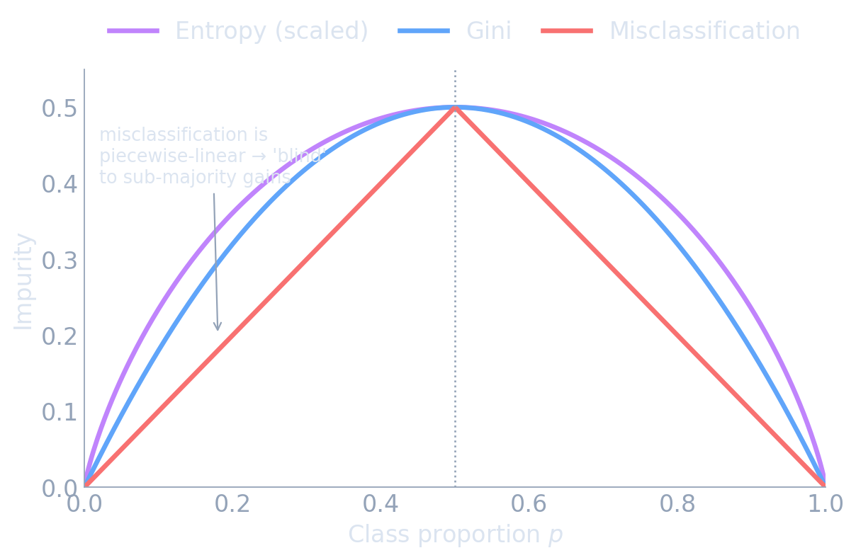
All three peak at \(p=0.5\) and vanish at pure nodes — but misclassification error is piecewise-linear, so it cannot reward a split that purifies a child without flipping its majority. Gini/entropy are strictly concave and can.

• Gini and entropy give very similar trees in practice; Gini is slightly cheaper (no log) and is the scikit-learn default.
• Misclassification error is not used for growing — it is insensitive to changes that don’t flip the majority class.

• The examinable insight: for regression, “impurity = variance” means a regression tree is doing piecewise least squares — it connects directly back to the MSE/Gaussian story of Unit 7. Say “the tree is least squares with a learned partition.”
• Why not misclassification error for splitting? Concrete example: a 400/100 node split into 300/0 and 100/100 — misclassification error is unchanged (still 100 errors) but Gini/entropy both drop sharply. The curvature of Gini/entropy rewards purer children even without a majority flip. This is a classic exam question — drill it.
• Don’t over-spend here (~3 min). The takeaway is “Gini ≈ entropy, both are concave purity measures; variance for regression.” Move on.

Growing and pruning a tree

• Grow: recurse until a stopping rule — max depth, min samples per leaf, or no positive impurity gain.
• An unconstrained tree grows until every leaf is pure → it memorizes the training set (zero training error).
• Pre-pruning (early stopping): cap depth / min-leaf-size. Cheap but myopic — a weak split may enable a strong one below it.
• Post-pruning (cost-complexity): grow fully, then prune back minimizing \(R_\alpha(T)=R(T)+\alpha|T|\) — error plus a penalty on the number of leaves.

• Make the regularization parallel explicit: cost-complexity pruning \(R(T)+\alpha|T|\) is exactly the regularized-ERM template from Unit 7 — fit quality plus a complexity penalty, with \(\alpha\) tuned by cross-validation. Trees are not exempt from the bias–variance law; pruning is their λ.
• Practical reality check for the materials audience: in modern practice you almost never carefully prune a single tree — you let trees overgrow and control complexity at the ensemble level (RF: fully grown; GBM: shallow + shrinkage + early stopping). Pruning matters conceptually and for single-tree interpretability, not for production accuracy.
• The “pre-pruning is myopic” point motivates why fully-grown-then-ensemble beats carefully-pruned-single — bridge to the next slides.

A single tree is a high-variance learner

• Stop too early → underfit (high bias, low variance).
• Grow to pure leaves → near-zero training error (low bias, high variance).
• A small change in the training data can completely reshape a deep tree — the greedy top split flips and the whole structure changes.
• Pruning trades some variance for bias, but a single tree never escapes this instability.

This is precisely the regime where averaging helps. → Ensembles.

• This slide is the hinge of the unit — it places the single tree in the high-variance corner of the bias–variance picture and thereby motivates the entire rest of the lecture. Point at the “↓Var” arrow on the board.
• Make instability visceral: deep trees are so sensitive that re-sampling the data or removing one influential point can change the root split and cascade. That sensitivity is not a bug to fix by pruning — it is the raw material bagging exploits (averaging unstable, decorrelated predictors is exactly what reduces variance).
• One-line bridge: “A single tree is the best possible input to an averaging machine — low bias, high variance, fast to train. Now let’s average.”

Strengths and limitations of a single tree

Strengths

• Interpretable (you can read the rules).
• No scaling / encoding ceremony; handles missing values.
• Captures interactions and nonlinearity automatically.
• Fast, \(O(N d\log N)\).

Limitations

• High variance / unstable.
• Piecewise-constant: no smooth extrapolation.
• Greedy → not globally optimal.
• Axis-aligned → diagonal structure needs many splits.

• This is the honest scorecard; every limitation on the right is addressed (or inherited) by ensembles, so frame it as the agenda for the next two sections: variance → bagging/RF; bias from shallow/greedy → boosting; the piecewise-constant/axis-aligned limits are inherent and resurface at the trees-vs-NN comparison.
• The interpretability strength is the one ensembles partially sacrifice — flag it now and promise the resolution (TreeSHAP, importance) in the interpretability slide. Materials reviewers and regulators care about this; it’s not academic.
• Keep brief (~2 min); it is a consolidation slide before the first interactive.

Interactive: tree depth controls the fit

• A 1D regression tree fit to noisy data \(y=\sin(2x)+0.3x+\varepsilon\).
• Drag max depth: depth 1 = one stump (high bias); large depth = a step for almost every point (high variance / memorization).

viewof tree_depth = Inputs.range([1, 10], {value: 3, step: 1, label: "Max depth"})
viewof tree_noise = Inputs.range([0, 0.8], {value: 0.3, step: 0.05, label: "Noise σ"})
viewof tree_reseed = Inputs.button("Resample data")

tree_data = {
  tree_reseed;
  const n = 60;
  const rnd = d3.randomNormal(0, tree_noise);
  const pts = [];
  for (let i = 0; i < n; i++) {
    const x = (i / (n - 1)) * 6;
    pts.push({ x, y: Math.sin(2 * x) + 0.3 * x + rnd() });
  }
  return pts;
}

function buildRegTree(rows, depth, maxDepth) {
  const ys = rows.map(d => d.y);
  const mean = d3.mean(ys);
  if (depth >= maxDepth || rows.length < 4) return { leaf: true, value: mean };
  const xs = Array.from(new Set(rows.map(d => d.x))).sort((a, b) => a - b);
  let best = null;
  for (let i = 1; i < xs.length; i++) {
    const thr = (xs[i - 1] + xs[i]) / 2;
    const L = rows.filter(d => d.x <= thr);
    const R = rows.filter(d => d.x > thr);
    if (L.length < 2 || R.length < 2) continue;
    const sse =
      L.length * (d3.variance(L.map(d => d.y)) || 0) +
      R.length * (d3.variance(R.map(d => d.y)) || 0);
    if (best === null || sse < best.sse) best = { thr, sse, L, R };
  }
  if (best === null) return { leaf: true, value: mean };
  return {
    leaf: false,
    thr: best.thr,
    left: buildRegTree(best.L, depth + 1, maxDepth),
    right: buildRegTree(best.R, depth + 1, maxDepth)
  };
}

function predictTree(node, x) {
  return node.leaf ? node.value : (x <= node.thr ? predictTree(node.left, x) : predictTree(node.right, x));
}

tree_fitted = {
  const t = buildRegTree(tree_data, 0, tree_depth);
  return d3.range(0, 6.001, 0.02).map(x => ({ x, y: predictTree(t, x) }));
}

Plot.plot({
  width: 820, height: 430,
  marginLeft: 60, marginBottom: 52, marginTop: 20,
  style: {
    background: "transparent",
    color: "#e5edf7",
    fontSize: "20px",
    fontFamily: "Inter, sans-serif"
  },
  x: { domain: [0, 6], label: "x →", grid: true },
  y: { domain: [-2, 3], label: "↑ y", grid: true },
  marks: [
    Plot.line(d3.range(0, 6.01, 0.05), { x: d => d, y: d => Math.sin(2 * d) + 0.3 * d, stroke: "#94a3b8", strokeDasharray: "4,4", strokeWidth: 2 }),
    Plot.dot(tree_data, { x: "x", y: "y", r: 3.5, fill: "#60a5fa", fillOpacity: 0.55 }),
    Plot.line(tree_fitted, { x: "x", y: "y", stroke: "#4ade80", strokeWidth: 3, curve: "step-after" })
  ]
})

• Demo script (~90 s): start depth 1 — narrate “one split, gross underfit, pure bias.” Step to 3–4 — “captures the shape, good bias/variance balance.” Push to 10 — “a step per point, the orange line chases every noisy dot: that is variance/memorization.” Then hit Resample data at depth 10 — the fit reshapes completely; at depth 3 it barely moves. That contrast is the high-variance lesson, shown not told.
• The step-shaped fit makes the piecewise-constant nature undeniable — tie back to “trees can’t extrapolate smoothly.”
• Recovery point: 30 s suffices if behind; the single must-show is resample-at-high-depth vs resample-at-low-depth.

From one tree to many: the ensemble idea

• Averaging \(B\) predictors that are individually noisy but not making the same mistakes cancels their independent errors.
• For unbiased predictors, averaging leaves bias unchanged but shrinks variance.
• We need many trees that are (a) individually low-bias and (b) as decorrelated as possible.
• Two ways to build them: resample the data (bagging) and restrict the features (random forest).

• This is the conceptual core of bagging stated before any formula — make sure they get the intuition first: “errors that point in random directions cancel; bias points the same way every time, so averaging can’t remove it.” That single sentence predicts everything on the next three slides.
• The two requirements (low-bias base learner + decorrelation) are the design spec; bagging delivers the first via fully-grown trees, RF delivers the second via feature subsampling. Frame the next slides as “meeting this spec.”
• Connect to Unit 7’s variance-of-the-mean (\(\sigma^2/N\)) — averaging is the same statistical lever, now applied to predictors instead of measurements.

Bootstrap sampling

• A bootstrap sample: draw \(N\) points from the training set with replacement.
• Each bootstrap sample contains \(\approx 63\%\) of the unique points; the rest are duplicated.
• The omitted \(\approx 37\%\) are out-of-bag for that tree — a free held-out set (used later).
• Different bootstrap samples → different trees → the decorrelation we need.

• The 63%/37% numbers come from \(1-(1-1/N)^N \to 1-e^{-1}\approx 0.632\) — show the one-line limit; it’s a satisfying derivation and it makes OOB error (two slides on) feel principled rather than magical.
• Emphasize with replacement — sampling without replacement at size N would just return the whole set; the replacement is what injects the per-tree variation that decorrelates the ensemble.
• Bootstrap is also a Unit-7 callback (resampling to estimate variability) — name the continuity so the course feels cumulative.

Bagging — variance reduction by averaging

Bootstrap aggregating (Breiman 1996):

1. Draw \(B\) bootstrap samples (size \(N\), with replacement).
2. Train one fully grown tree per sample (low bias, high variance).
3. Predict by averaging: \(\hat f_{\text{bag}}(x)=\frac1B\sum_{b=1}^B \hat f_b(x)\) (regression) or majority vote (classification).

\[\mathrm{Var}\!\left(\tfrac1B\sum_b \hat f_b\right)=\rho\,\sigma^2+\frac{1-\rho}{B}\,\sigma^2.\]

As \(B\to\infty\) the second term vanishes; variance floors at \(\rho\sigma^2\).

• This formula is the intellectual center of the whole bagging/RF story — derive the two terms verbally: \(\sigma^2\) is one tree’s variance, \(\rho\) is the average pairwise prediction correlation. Term 2 (\(\propto 1/B\)) is killed by more trees; term 1 (\(\rho\sigma^2\)) is not — it is the floor.
• The punchline that motivates random forests on the very next slide: “throwing more trees at bagging hits a wall set by \(\rho\). To go lower you must reduce \(\rho\) itself.” Write the floor \(\rho\sigma^2\) on the board and box it.
• Note bias is absent from the formula by design — averaging unbiased trees does not touch bias. Reiterate the board arrow.

The correlation ceiling

• Trees trained on bootstrap samples of the same data still pick the same dominant splits → highly correlated predictions (\(\rho\) large).
• Large \(\rho\) ⇒ the \(\rho\sigma^2\) floor is high ⇒ bagging alone gives only modest gains.
• To break the ceiling we must force the trees to be structurally different — not just trained on resampled data.
• Random forests do this by restricting the features each split may consider.

• This slide exists to make the next one (RF) feel inevitable rather than arbitrary. The story: bagging is necessary but insufficient; the binding constraint is \(\rho\), and resampling data alone barely moves \(\rho\) because one or two strong features dominate the top splits in every tree.
• Materials-relevant intuition: if “annealing temperature” is by far the most predictive feature, every bagged tree splits on it first and they all look alike — bagging wastes its averaging on near-duplicates. Feature subsampling forces some trees to discover the secondary structure.
• Keep tight; it’s the logical bridge, ~2 min.

Random forest = bagging + random feature subsets

• At each split, search only a random subset of features (typical: \(\sqrt{d}\) for classification, \(d/3\) for regression).
• This decorrelates the trees (\(\rho\downarrow\)) → the \(\rho\sigma^2\) floor drops → averaging buys far more.
• Slight increase in individual-tree bias (each split sees fewer options), massively offset by the variance reduction.
• The de-facto default: RandomForestRegressor / RandomForestClassifier (Breiman 2001).

With \(B\approx 500\) fully grown, feature-subsampled trees, RF is a strong, low-tuning baseline that usually crushes a single tuned tree.

• Breiman’s 2001 insight in one sentence: “don’t just bag — also decorrelate, at every split.” Connect it explicitly to the boxed floor \(\rho\sigma^2\) from two slides ago: RF lowers \(\rho\), which lowers the floor; that is the entire mechanism.
• Be honest about the trade: restricting features raises each tree’s bias slightly. The reason RF still wins is that the variance term dominates for deep trees, so trading a little bias for a lot of decorrelation is hugely net-positive. This is bias–variance reasoning applied live — point at the board.
• Practical default to state: 500 trees, \(\sqrt d\) / \(d/3\) features, fully grown. RF’s reputation for “works well with almost no tuning” is real and worth emphasizing for the materials audience.

See it: averaging smooths the boundary

One deep tree carves jagged, memorised islands; averaging 200 decorrelated trees blends them into a smooth, stable boundary.

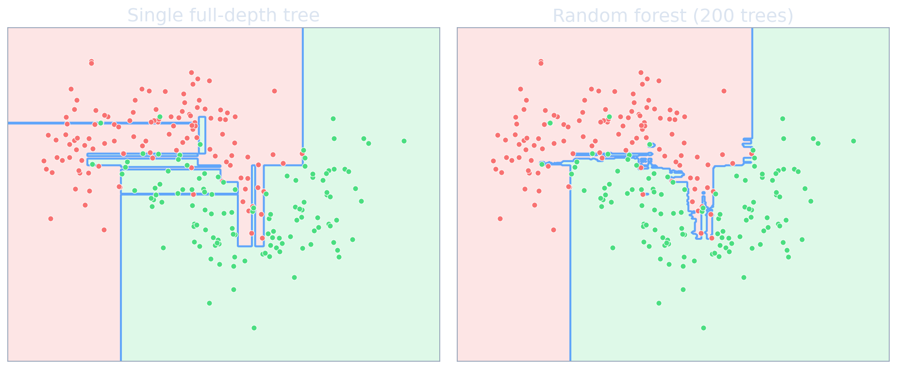
• Left = high variance: every noisy point gets its own box.
• Right = the same trees, averaged → the staircase washes out.
• The decision boundary barely moves if you resample the data — exactly the variance reduction the \(\rho\sigma^2\) formula promised.
• Bias is untouched; only the jitter is gone.

• This is the visual payoff of the whole bagging/RF section — pair it explicitly with the single-tree instability figure from §1: same kind of data, but averaging removes the fragility. “Remember the boundary that jumped around? Average 200 of them and it stops jumping.”
• Point out that the smooth boundary is not from lower-variance individual trees (each is still a jagged deep tree) — it emerges from averaging decorrelated jagged predictors. That is the entire mechanism, made visible.

Interactive: the bagging variance ceiling

• Plot of ensemble variance \(\;\rho\sigma^2+\frac{1-\rho}{B}\sigma^2\;\) (with \(\sigma^2=1\)) vs number of trees \(B\).
• See the floor at \(\rho\sigma^2\): lowering correlation (what random forests do) is what actually buys you accuracy.

viewof rho_a = Inputs.range([0.0, 1.0], {value: 0.6, step: 0.02, label: "ρ (bagging)"})
viewof rho_b = Inputs.range([0.0, 1.0], {value: 0.15, step: 0.02, label: "ρ (random forest)"})

ens_var = (rho, B) => rho + (1 - rho) / B;

var_curves = {
  const rows = [];
  for (let B = 1; B <= 200; B++) {
    rows.push({ B, v: ens_var(rho_a, B), kind: `Bagging (ρ=${rho_a.toFixed(2)})` });
    rows.push({ B, v: ens_var(rho_b, B), kind: `Random forest (ρ=${rho_b.toFixed(2)})` });
  }
  return rows;
}

Plot.plot({
  width: 1000, height: 700,
  marginLeft: 80, marginBottom: 64, marginTop: 50,
  style: {
    background: "transparent",
    color: "#e5edf7",
    fontSize: "21px",
    fontFamily: "Inter, sans-serif"
  },
  x: { domain: [1, 200], label: "Number of trees B →", grid: true },
  y: { domain: [0, 1], label: "↑ Ensemble variance (σ²=1)", grid: true },
  color: { legend: true, range: ["#f87171", "#60a5fa"] },
  marks: [
    Plot.ruleY([rho_a], { stroke: "#f87171", strokeDasharray: "4,4", strokeWidth: 1.5 }),
    Plot.ruleY([rho_b], { stroke: "#60a5fa", strokeDasharray: "4,4", strokeWidth: 1.5 }),
    Plot.line(var_curves, { x: "B", y: "v", stroke: "kind", strokeWidth: 3.5 })
  ]
})

• Demo (~60 s): with both ρ’s default, both curves drop fast then flatten — onto their dashed floors. Drag “ρ (bagging)” up to 0.9: the red floor barely moves with B — “more trees, no gain; you are stuck on the ceiling.” Drag “ρ (random forest)” toward 0: the blue floor collapses — “this is what RF buys, and it’s a property of decorrelation, not of B.”
• The single takeaway to verbalize: after ~100 trees, adding more is nearly free of benefit; the lever that matters is ρ. This also explains the standard advice “≥ a few hundred trees, then stop tuning B.”
• Tie back to the boxed formula; this interactive is that formula made tactile.

Out-of-bag (OOB) error

• Each tree’s bootstrap sample omits \(\approx37\%\) of points — its out-of-bag set.
• Predict each training point using only the trees that did not see it, then score.
• Result: a nearly free, CV-quality estimate of generalization error — no separate validation split needed.
• OOB curves vs \(B\) also tell you when adding trees has stopped helping.

• OOB is one of the most under-used diagnostics in applied tabular ML — emphasize it for the materials audience, where data is scarce and giving up a validation split hurts. “RF hands you a held-out estimate for free; use it.”
• Be precise about the mechanism so they can implement it: a point’s OOB prediction aggregates only the ~37% of trees for which it was out-of-bag. With enough trees this is a legitimate generalization estimate, empirically close to k-fold CV but at a fraction of the cost.
• Caveat to state: OOB error degrades under the same assumption-violations as CV (e.g., grouped/temporal structure, distribution shift) — it is not magic, it is CV’s cheaper cousin. Bridge to the conformal caveat from Unit 7 if students ask.

Impurity (MDI) importance — what it measures

MDI = Mean Decrease in Impurity. Reuse the per-split gain \(\Delta\) from “how splits are chosen”: credit each feature with the impurity it removed, weighted by how many samples passed through that split, summed over every node and averaged across all \(B\) trees.

\[ \text{MDI}_j \;=\; \frac{1}{B}\sum_{b=1}^{B}\;\sum_{\substack{\text{nodes in tree }b\\\text{that split on }j}} \frac{N_{\text{node}}}{N}\,\Delta_{\text{node}}, \qquad \text{then normalized so } \sum_j \text{MDI}_j = 1. \]

• It is feature_importances_ in scikit-learn — free, computed during training, no extra passes.
• Computed on the training set → it cannot tell “genuinely useful” from “useful for memorizing.”
• Cardinality bias: a continuous / high-cardinality column offers more candidate thresholds, so it wins more splits and accumulates spurious \(\Delta\) — even pure noise scores nonzero.

• Spell the formula out loud: “for each split on feature \(j\), take its impurity drop \(\Delta\), scale by the fraction of samples reaching that node, add them all up over every tree, normalize.” The sample-weighting is the part students miss — a split near the root that sorts many samples counts far more than a deep split touching ten points.
• The two failure causes to name explicitly: (1) it’s a training-set quantity (no held-out check), (2) cardinality bias — more thresholds = more chances to reduce impurity by chance. These are exactly what the worked example two slides on will show.
• This slide exists so “MDI is biased” on the next slide is a conclusion students can derive, not a claim they must accept.

Feature importance — done right

Impurity (Gini/MDI) importance

• Sum of (sample-weighted) impurity reduction per feature across all splits and trees, normalized to 1.
• Free, but biased: inflates high-cardinality / continuous features and is unreliable under correlated features.

Better alternatives

• Permutation importance: shuffle one feature, measure the performance drop on held-out data (explained next). Model-agnostic, honest.
• TreeSHAP (Lundberg et al. 2020): exact Shapley values for trees — consistent, local + global.

For a materials paper claiming “feature X drives the property,” report permutation or SHAP, not raw impurity importance.

• This is the slide that prevents a real, common scientific error. Materials papers routinely publish RF impurity-importance bar charts as if they were causal feature rankings; impurity importance is biased toward high-cardinality and continuous features and is destabilized by correlated descriptors (ubiquitous in compositional data). Say bluntly: “do not put impurity importance in a paper as evidence.”
• Give the actionable rule: permutation importance for an honest global ranking, TreeSHAP when you need per-sample explanations or correlated-feature robustness. This is also the explicit bridge to Unit 14 (explainability) — name it.
• None of these are causal — importance ≠ causation. Add the one-sentence caveat; it’s the second most common misuse.
• The next two slides unpack permutation importance (which students have not seen) and show the impurity-vs-permutation failure on a worked example.

Permutation importance — how it actually works

It answers one question: how much does the trained model actually rely on this feature?

1. Score the fitted model on a held-out set (e.g. \(R^2\) or accuracy) → baseline.
2. Take one feature and randomly shuffle its column across rows. The column keeps its distribution but its link to the target is destroyed.
3. Re-score the same model on the shuffled data.
4. Importance = baseline − shuffled score — the bigger the drop, the more the model needed that feature.
5. Repeat the shuffle a few times and average (it is random).

• Intuition: if scrambling a feature barely hurts, the model was not using it; if the score collapses, it was load-bearing.
• Model-agnostic: works for any fitted model (RF, GBM, neural net) — it only needs predict and a score.
• Computed on held-out data, so it cannot be fooled by training-set overfitting — the key advantage over impurity (MDI) importance.
• Caveat: two correlated features can share importance — shuffle one and its twin still leaks the signal, so both look weak. Group them, or use SHAP.

• Define it concretely because students have never seen it: “permute = shuffle the column.” Do the one-sentence thought experiment live — “imagine I randomly reassign every alloy’s Cr value to a different alloy; if the model’s error barely moves, the model wasn’t really using Cr.”
• Stress the held-out point: this is why permutation beats MDI — MDI is a training-set quantity and cannot tell whether a feature helped genuinely or just helped memorize. Permutation asks the test set.
• The correlation caveat is the one honest limitation to state so they don’t over-trust it on compositional data where features are simplex-constrained and correlated.

Example: impurity importance is fooled by noise

Same random forest, same data, two ways of scoring features. A column of pure noise earns as much impurity (MDI) importance as a genuine weak feature — MDI is computed on the training set and rewards the many spurious splits a high-cardinality column enables. Permutation importance on held-out data correctly assigns the noise ≈ 0.

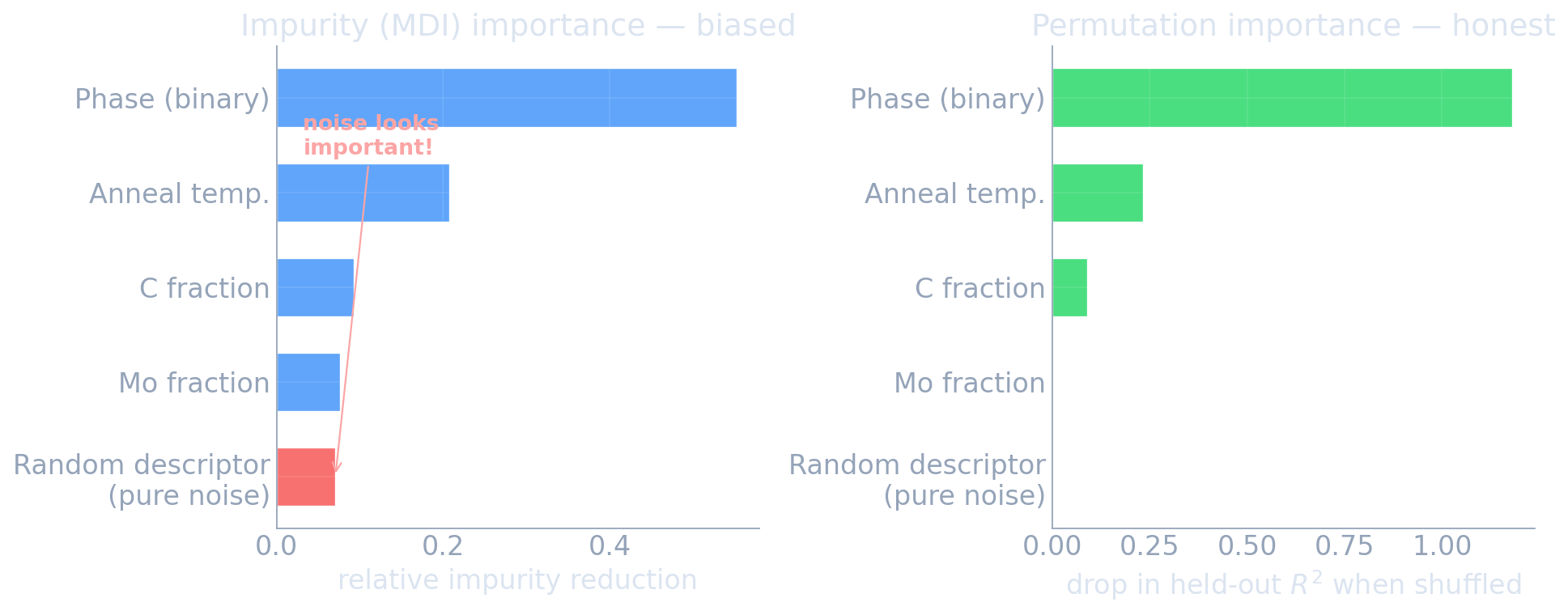
• Left (MDI): the random descriptor ranks alongside real Mo fraction — a red flag you would never catch from the bar chart alone.
• Right (permutation): the noise and the genuinely-useless Mo both drop to ≈ 0.
• Both panels agree the real driver is Phase, then anneal temp, then C.
• Lesson: never publish raw MDI as evidence that a feature “matters.”

• This is the payoff: a concrete, reproducible failure of the default feature_importances_. The noise column is literally np.random.uniform and never enters the target, yet MDI gives it real-feature-level importance because (a) it is computed on train and (b) continuous high-cardinality columns offer more thresholds to overfit.
• Walk left→right: “MDI says noise ≈ Mo; permutation on held-out says noise = 0. The second one is telling the truth.” This single picture justifies the whole slide’s rule.
• Numbers are real (scikit-learn permutation_importance), not illustrative — say so; it pre-empts “did you cook this?” and models honest reporting.

Extremely randomized trees (ExtraTrees)

• Like a random forest, but the split threshold is chosen at random (not optimized) for each candidate feature.
• Even more decorrelation (\(\rho\) even lower) → lower variance, slightly higher bias.
• Often trains faster (no threshold search) and can match RF on noisy tabular data (Geurts et al. 2006).
• A useful second baseline to try alongside RF — one line to swap in scikit-learn.

• Keep this brief (~2 min) — it is a “know it exists, it’s one import away” slide, not a deep topic. The conceptual value: it shows the decorrelation lever taken to its logical extreme (randomize even the threshold), reinforcing the ρ-is-the-thing message.
• Practical guidance: try RF and ExtraTrees both as quick baselines; ExtraTrees sometimes wins on very noisy materials measurements and is cheaper to fit. Not usually the final model — that’s typically gradient boosting (next section).

Random forest in practice

• Hyperparameters that matter: number of trees \(B\) (more = better then flat), min samples per leaf, max features per split.
• Hyperparameters that mostly don’t: tree depth (let them grow), splitting criterion.
• Use OOB (or CV) to pick min-leaf and max-features; set \(B\) as large as your compute allows.
• Strong, robust, low-effort baseline — but for peak tabular accuracy, boosting usually wins (next).

• The actionable summary: RF is the “first model you run” — minimal tuning, robust, gives you OOB error and importances for free. It is the baseline every materials project should start from before anything fancier.
• Reiterate the asymmetry: depth and criterion barely matter (fully grown + Gini/variance is fine); min-leaf and max-features are the knobs, tuned via OOB. This saves students from wasted grid searches.
• Transition line into boosting: “RF squeezes out variance and then plateaus. To push accuracy further we stop averaging independent trees and start composing dependent ones — boosting.” Point at the board’s ↓Bias arrow.

Boosting — sequential bias reduction

• Bagging/RF: average many low-bias, high-variance trees in parallel → cut variance.
• Boosting: build a sequence of high-bias, low-variance weak learners (shallow trees), each correcting the previous ensemble’s errors.
• Additive model: \(\hat f^{(t)}(x)=\hat f^{(t-1)}(x)+\eta\,h_t(x)\).
• Bias falls as the ensemble grows — the opposite mechanism to bagging.

Bagging averages independent learners; boosting composes dependent ones.

• The parallel-vs-sequential, variance-vs-bias contrast is the single most important conceptual takeaway of the boosting section. Put it as a 2×2 on the board: {bagging/RF: parallel, ↓Var, deep trees} vs {boosting: sequential, ↓Bias, shallow trees}. Every student should be able to reproduce this table in the exam.
• Stress why shallow weak learners: a boosting step only needs to nudge the ensemble toward the residual; a deep tree as the weak learner would overfit each step and the sequence would not generalize. Depth 3–6 stumps/trees is the norm — the bias is intentional and is removed by the sequence, not by each member.
• Historical one-liner: AdaBoost (1997) launched the field; everything modern is gradient boosting — next two slides.

AdaBoost — the original idea

• Maintain a weight on each training point; start uniform.
• Each round: fit a weak learner, up-weight the misclassified points, down-weight the correct ones.
• Final prediction: weighted vote of all weak learners, better learners weighted more (Freund and Schapire 1997).
• Reframed later (Friedman): AdaBoost is gradient boosting with an exponential loss — a special case of the general view next.

• Keep this historical and short (~3 min). Its pedagogical job: give an intuitive, weights-based picture of “focus on what you’re getting wrong” before the more abstract functional-gradient formulation. Many students grok AdaBoost’s reweighting first, then see gradient boosting as its generalization.
• The key bridge sentence: “re-weighting misclassified points is, mathematically, taking a step against the gradient of an exponential loss.” That reframing (Friedman 2001) is exactly the next slide — set it up here so the generalization lands.
• Note AdaBoost is rarely used directly today (sensitive to noisy labels/outliers via the exponential loss); it’s the conceptual ancestor, not the production tool.

Gradient boosting — descent in function space

• Think of the predictor \(\hat f\) itself as the thing being optimized — not a parameter vector, but a function.
• We want to minimize \(\sum_i \mathcal{L}(y_i,\hat f(x_i))\). The steepest-descent direction at each point is the negative gradient of the loss w.r.t. the prediction.
• We cannot store an arbitrary function — so fit a tree to approximate that negative-gradient direction, and take a small step along it.
• Gradient boosting = gradient descent, where each step is a regression tree (Friedman 2001).

• This is the “aha” slide of the section — deliver it with weight. The analogy to Unit 6 is exact and worth drawing: there, gradient descent moved a parameter vector \(\theta\) against \(\nabla_\theta L\); here it moves a function \(\hat f\) against \(\nabla_{\hat f} L\), and because we can’t represent arbitrary functions we project the gradient onto “the space of trees” by fitting a tree to it.
• The learning rate η is literally the same η as Unit 6 — the step size of functional gradient descent. Foreshadow that “small η + many steps” will be the same speed/stability story as the optimizer unit (it is).
• If students only remember one sentence: “boosting is gradient descent and the trees are the steps.” Everything operational (pseudo-residuals, shrinkage, early stopping) follows from that.

Gradient boosting — the algorithm

For loss \(\mathcal{L}\), at iteration \(t\):

1. Pseudo-residuals: \(r_i^{(t)}=-\dfrac{\partial \mathcal{L}(y_i,\hat f^{(t-1)}(x_i))}{\partial \hat f^{(t-1)}(x_i)}\).
2. Fit a small regression tree \(h_t\) to predict \(r_i^{(t)}\).
3. Update: \(\hat f^{(t)}=\hat f^{(t-1)}+\eta\,h_t\).

\(\eta\) = learning rate (shrinkage). Small \(\eta\) + many trees generalizes better than large \(\eta\) + few.

• Walk the three steps as “compute the direction (gradient), approximate it with a tree, take a small step” — explicitly mapping each to the functional-gradient picture from the previous slide so it is not three memorized lines.
• The shrinkage point is the most important practical rule in the section: η small (0.01–0.1) with many trees (hundreds–thousands) + early stopping is the standard recipe; large η is faster but overfits and is less robust. This is the same speed/stability trade-off as Unit 6’s learning rate — say so explicitly, it consolidates the course.
• Set up the next slide: “what are these pseudo-residuals concretely? For squared error they’re something you already know.”

See it: the ensemble builds up tree by tree

Fitting \(y=\sin 2x+0.3x+\varepsilon\). Each panel adds more shrunken trees; the green ensemble grows from a crude step toward the dashed target. By 50 trees it starts chasing noise — why we early-stop.

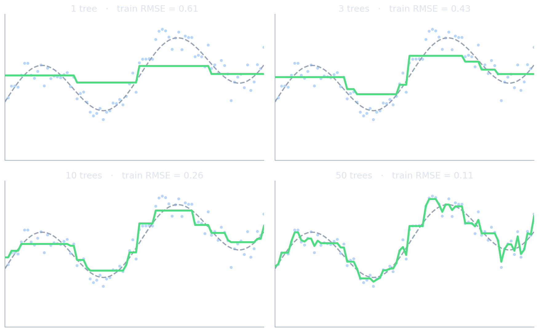
• 1 tree: one step — pure bias, just like a stump.
• 3–10 trees: the shape emerges as each tree fits the leftover residual.
• 50 trees: near-perfect on train — and beginning to wiggle on noise (variance creeping in).
• Bias falls monotonically; early stopping decides when to quit.

• The static companion to the boosting interactive: here you see the function being assembled, not just the RMSE curve. Walk left-to-right and narrate “each green curve = previous green curve + one shrunken tree fit to what was still wrong.”
• Tie the 50-tree wiggle to the regularization slide: this is the overfitting that early stopping / shrinkage exist to control. The same picture as Unit 6’s “train loss keeps falling while validation turns up.”

Pseudo-residuals — a worked example

Squared error \(\mathcal{L}=\tfrac12 (y-\hat f)^2\)

• \(-\partial\mathcal{L}/\partial\hat f = (y-\hat f)\).
• Pseudo-residual = ordinary residual.
• Each tree just fits “what the ensemble still gets wrong.”

Logistic / other losses

• The gradient gives a re-weighted target that focuses on hard, informative points.
• Same algorithm, only step 1 changes → boosting works for regression, classification, ranking, survival, custom losses.

• The squared-error case is the one to anchor: “fit a tree to the residuals, add a shrunk version, repeat” — this is the entire algorithm with no calculus, and it’s correct. Many students carry this picture forever; give it to them cleanly.
• Then the generalization: only step 1 (the gradient) changes for other losses; steps 2–3 are identical. That modularity is why gradient boosting is a framework, not one algorithm — and why XGBoost/LightGBM can support arbitrary differentiable objectives, including physics-informed custom losses in materials work.
• Connect to Unit 7: choosing the loss = choosing the noise model (Gaussian→squared error, Bernoulli→logistic). The “which loss” decision they learned there directly selects the pseudo-residual here.

Regularizing gradient boosting

Boosting can and will overfit — it drives training loss toward zero. Controls:

• Shrinkage \(\eta\): smaller steps, more trees — the primary regularizer.
• Number of trees + early stopping on a validation/OOB curve.
• Tree size: shallow trees (depth 3–6) cap interaction order and variance.
• Stochastic boosting: subsample rows and/or columns per tree (à la RF) → decorrelation + speed.
• Explicit penalties: L1/L2 on leaf values (XGBoost — next slide).

• Correct the most common misconception head-on: students think “boosting reduces bias, so it can’t overfit.” It absolutely overfits — unbounded boosting interpolates the training data. The bias↓ comes with variance↑ as t grows; early stopping is non-negotiable.
• The hierarchy of knobs to teach: η + early stopping first (biggest lever), then tree depth, then subsampling, then leaf penalties. This ordering is the practical tuning recipe two slides on — preview it.
• Stochastic gradient boosting (row/col subsampling) is the elegant point: it imports RF’s decorrelation trick into boosting, so the two families are not opposites but composable ideas. Reinforces the unit’s “everything is a bias–variance move” thesis.

Interactive: boosting iterations × learning rate

• Gradient-boosted stumps on the same \(y=\sin(2x)+0.3x+\varepsilon\) data.
• Watch train vs validation RMSE: large \(\eta\) overfits fast; small \(\eta\) needs more rounds but generalizes better.

viewof gb_eta = Inputs.range([0.02, 1.0], {value: 0.3, step: 0.02, label: "Learning rate η"})
viewof gb_T = Inputs.range([1, 120], {value: 40, step: 1, label: "Number of trees"})

gb_all = {
  const n = 70;
  const rndTr = d3.randomNormal(0, 0.3);
  const rndVa = d3.randomNormal(0, 0.3);
  const tr = [], va = [];
  for (let i = 0; i < n; i++) {
    const x = (i / (n - 1)) * 6;
    tr.push({ x, y: Math.sin(2 * x) + 0.3 * x + rndTr() });
    const xv = ((i + 0.5) / n) * 6;
    va.push({ x: xv, y: Math.sin(2 * xv) + 0.3 * xv + rndVa() });
  }
  return { tr, va };
}

bestStump = function (rows) {
  const xs = Array.from(new Set(rows.map(d => d.x))).sort((a, b) => a - b);
  let best = null;
  for (let i = 1; i < xs.length; i++) {
    const thr = (xs[i - 1] + xs[i]) / 2;
    const L = rows.filter(d => d.x <= thr);
    const R = rows.filter(d => d.x > thr);
    if (!L.length || !R.length) continue;
    const cL = d3.mean(L, d => d.r), cR = d3.mean(R, d => d.r);
    let sse = 0;
    for (const d of L) sse += (d.r - cL) ** 2;
    for (const d of R) sse += (d.r - cR) ** 2;
    if (best === null || sse < best.sse) best = { thr, cL, cR, sse };
  }
  return best;
}

gb_curves = {
  const { tr, va } = gb_all;
  const stumps = [];
  let predTr = tr.map(() => 0);
  let predVa = va.map(() => 0);
  const rmse = (arr, pred) => Math.sqrt(d3.mean(arr.map((d, i) => (d.y - pred[i]) ** 2)));
  const rows = [];
  for (let t = 1; t <= gb_T; t++) {
    const resid = tr.map((d, i) => ({ x: d.x, r: d.y - predTr[i] }));
    const s = bestStump(resid);
    if (!s) break;
    stumps.push(s);
    predTr = tr.map((d, i) => predTr[i] + gb_eta * (d.x <= s.thr ? s.cL : s.cR));
    predVa = va.map((d, i) => predVa[i] + gb_eta * (d.x <= s.thr ? s.cL : s.cR));
    rows.push({ t, e: rmse(tr, predTr), kind: "Train RMSE" });
    rows.push({ t, e: rmse(va, predVa), kind: "Validation RMSE" });
  }
  return rows;
}

Plot.plot({
  width: 820, height: 430,
  marginLeft: 64, marginBottom: 52, marginTop: 44,
  style: {
    background: "transparent",
    color: "#e5edf7",
    fontSize: "20px",
    fontFamily: "Inter, sans-serif"
  },
  x: { domain: [1, gb_T], label: "Boosting iteration →", grid: true },
  y: { domain: [0, 1.2], label: "↑ RMSE", grid: true },
  color: { legend: true, range: ["#60a5fa", "#f87171"] },
  marks: [
    Plot.line(gb_curves, { x: "t", y: "e", stroke: "kind", strokeWidth: 3.5 })
  ]
})

• Demo (~90 s): η=0.3, 40 trees — train and validation both fall, validation flattens: healthy. Crank η→1.0: train RMSE plummets toward 0 while validation turns up — textbook overfitting; point at the divergence and say “this gap is variance; this is why you early-stop.” Then set η=0.05 and push trees to 120: slower descent, but train and validation track together far longer — the shrinkage lesson, shown.
• The single takeaway: the validation minimum is where you stop; small η widens and flattens that basin, making the stopping point forgiving. This is the same speed/stability picture as Unit 6’s learning rate — call back to it.
• Robustness: stumps keep it fast and the curves stable; if behind, 30 s on the η=1.0 overfit divergence is the must-show.

XGBoost — the regularized objective

• Optimizes a second-order Taylor expansion of the loss at each step (uses gradient and Hessian) → better steps, principled leaf values.
• Adds an explicit complexity penalty: \(\Omega(h)=\gamma T+\tfrac12\lambda\lVert w\rVert^2\) (number of leaves \(T\), leaf weights \(w\)).
• Histogram-based split finding: bin features → near-linear-time training on large data.
• Native missing-value handling, column/row subsampling, parallel + GPU (Chen and Guestrin 2016).

This is why XGBoost, not plain gradient boosting, is the general-purpose tabular workhorse — and the most documented one.

• The conceptual upgrade over Friedman’s GBM: XGBoost uses the second-order expansion (Newton-style step in function space), so the leaf values are computed from gradient and curvature rather than a line search — better-conditioned steps, which is a direct callback to the second-order discussion in Unit 6.
• The \(\gamma T+\tfrac12\lambda\|w\|^2\) penalty is the regularized-ERM template from Unit 7 applied to trees: penalize number of leaves (structure) and leaf magnitudes (L2). Say “trees are not exempt from regularization; XGBoost just bakes it into the objective.” This is the slide that earns its place vs the old one-bullet treatment.
• Histogram splits are the engineering reason it’s fast enough to be a default — not a conceptual point, but the one that made boosting practical at scale; LightGBM pushes this further (next slide).

CatBoost — the materials-tabular default

Three ideas, all aimed at categorical-heavy, modest-size tabular data (Prokhorenkova et al. 2018):

• Ordered target statistics: encode a category using only earlier rows’ targets → native categoricals, no target leakage, no manual one-hot.
• Ordered boosting: score each model on rows it did not train on → removes the prediction-shift bias all other GBMs carry.
• Oblivious (symmetric) trees: the same split across a whole level → strong implicit regularization + very fast inference.

• Best out-of-the-box accuracy with almost no tuning — the decisive property for non-experts.
• Native handling of the categoricals that fill materials data: alloy family, processing route, crystal system, phase.
• GPU support; robust on the few-hundred-to-tens-of-thousands-row regime typical here.
• Honest caveat: XGBoost has the larger ecosystem/docs; LightGBM is faster at very large \(N\).

For the typical materials problem, start with CatBoost. Reach for XGBoost as the general-purpose workhorse, LightGBM when \(N>10^6\).

• This is the slide that changes their default modeling choice — deliver the rationale, not just the name. The decisive argument for this cohort: CatBoost rewards not being a tuning expert. XGBoost’s ceiling is reached only with skilled tuning; CatBoost is near that ceiling at defaults. For materials engineers who are not ML specialists, “great with defaults” beats “greater if you’re an expert.”
• The two mechanisms that matter for materials data: (1) ordered target statistics — explain the leakage it prevents: naive target/mean encoding of “alloy family” uses each row’s own label, silently inflating R²; CatBoost’s “use only prior rows” permutation fixes this. Students will otherwise make this exact mistake. (2) Ordered boosting — same permutation idea applied to the gradient step, removing prediction shift.
• Keep oblivious trees to one sentence (same split per level → regularization + fast inference); it’s the “why it’s also fast” footnote, not the headline.
• Be honest about the caveat so it’s not salesmanship: if there are no categoricals and you have tuning budget and a huge ecosystem need, XGBoost is at least as good. The recommendation is audience-conditioned, and saying so is good scientific hygiene.

Background: target (mean) encoding For a categorical like alloy_family ∈ {Ni-superalloy, 316L-stainless, Ti-6Al-4V, …}, you don’t want one-hot columns (too many, sparse). A powerful alternative is target encoding: replace each category with the average target value of rows in that category.

LightGBM — when speed matters

• Leaf-wise growth: always split the highest-loss leaf (not level-wise) → faster loss reduction per tree.
• GOSS (gradient-based one-side sampling) + EFB (exclusive feature bundling) → trains fast on \(N>10^6\) and wide sparse data.
• Trade-off: leaf-wise trees can become deep and unbalanced → overfits small data; guard with num_leaves cap / larger min_data_in_leaf.
• Same gradient-boosting framework as XGBoost — the difference is engineering, not theory (Ke et al. 2017).

• Frame all three GBMs as one algorithm with different engineering trade-offs, not three theories — XGBoost (robust general default + biggest ecosystem), CatBoost (best no-tuning + categoricals → materials default), LightGBM (speed at large N). That triangulation is the photographable mental model.
• The one practical warning students must hear: leaf-wise growth is exactly why LightGBM overfits small datasets — the typical materials dataset is small, so LightGBM is usually not the right pick here despite its speed reputation. Give the concrete guards (num_leaves, min_data_in_leaf) for when they do use it on large data.
• Don’t deep-dive GOSS/EFB mechanics (one sentence each); the objective is “know which to reach for and why,” not re-implement them.

A practical GBM tuning recipe

1. Start: \(\eta=0.1\), depth 4–6, subsample 0.8, colsample 0.8, large n_estimators.
2. Use early stopping on a validation set to pick the number of trees.
3. Tune tree depth and min child weight (capacity) next.
4. Lower \(\eta\) (e.g. 0.03) and raise n_estimators for the final model.
5. Tune L1/L2 leaf penalties last; re-confirm with cross-validation.

This recipe is mainly for XGBoost/LightGBM. CatBoost is usually near-optimal at its defaults — fit it first, only tune if it underperforms.

• This is the slide students should photograph and literally follow in the exercise and their theses. The ordering matters: early stopping first (it makes everything else cheaper and prevents you tuning on an overfit model), capacity second, shrinkage refinement last.
• The meta-lesson: change one thing at a time and always confirm on held-out / CV — the same experimental-hygiene rule from the Unit 6 optimizer guide. Consistency across units is intentional; point it out.
• Reassure them: GBMs have many knobs but the defaults are good; this recipe is “sensible defaults + early stopping,” not a 50-trial grid search. Over-tuning is a more common student error than under-tuning.

Trees vs neural networks on tabular data

Trees / boosting win when

• Tabular features (compositions, parameters).
• \(N \lesssim 10^5\) rows.
• Mixed types, missing values.
• Strong interactions, weak geometric structure.
• You need fast training + importances.

Neural networks win when

• Spatial / sequential / graph data.
• \(N \gg 10^5\).
• A pretrained foundation model exists (Unit 9).
• End-to-end from raw signals/images.

For most materials projects with tabular features: try gradient boosting first.

• This is the single most actionable slide of the unit for a working materials engineer. State the default unambiguously: tabular features → start with a gradient-boosted tree (CatBoost first for this cohort’s categorical-heavy data, XGBoost as the general workhorse); only reach for a NN when the data shape (images, spectra, sequences, graphs) demands it.
• Pre-empt the prestige bias: students assume deep learning is “more advanced” hence better. On tabular data that is empirically false (next slide quantifies it). Detaching “newer/deeper” from “better-for-this-problem” is a real learning objective.
• Bridge: “why do trees win on tabular? It’s not an accident — there are three concrete reasons.” → next slide.

Why tree ensembles still beat deep learning on tabular

• Robust to uninformative features: trees ignore them via split selection; MLPs must learn to.
• Non-smooth targets: real tabular targets have sharp thresholds/jumps — piecewise-constant trees fit these naturally; smooth MLPs fight them.
• Rotation non-invariance is a feature: trees respect the original, meaningful axes (each column is a physical quantity); MLPs are rotation-invariant and waste capacity.
• Empirically confirmed across 45 datasets (Grinsztajn et al. 2022).

• These three reasons are the intellectual payoff — and they are callbacks to the geometry slide (axis-aligned boxes) and the piecewise-constant point from the trees section. The deck has been building to this; make the callback explicit (“remember the staircase? on tabular data the staircase is correct”).
• The rotation point is the deepest and most counter-intuitive: NN rotation-invariance, an asset for images, is a liability for tabular data where columns are individually meaningful physical quantities (at% Cr, anneal °C). Mixing them via a learned rotation destroys structure trees exploit for free.
• Cite Grinsztajn 2022 as the empirical backbone (45 datasets) so this is evidence, not opinion. Sets up the honest exception: TabPFN, next.

See it: why rotation matters

Same points, same labels. On the original (meaningful) axes the forest finds a clean boundary in one cut. Rotate the data 45° and the same boundary now demands a ragged staircase of many splits — wasted capacity and worse generalization.

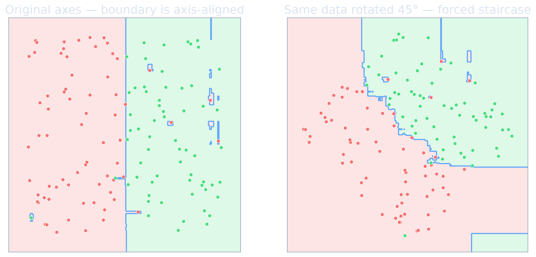
• Each column here is a physical quantity (at% Cr, anneal °C) — the informative cuts are axis-aligned.
• Trees exploit that for free; a rotation destroys it.
• A neural net is rotation-invariant — great for pixels, a liability when axes are meaningful.
• This is why “rotation non-invariance is a feature” for tabular data.

• This is the deck’s intellectual climax made visible — the explicit callback the previous notes promised: “remember the staircase from §1? On tabular data, where columns are meaningful, the staircase is correct and cheap; rotating the data is what makes trees struggle.”
• Drive the counter-intuition: students assume invariances are always good (they help on images). Here invariance is harmful because it discards the human-meaningful coordinate system. That reframing is the learning objective.

TabPFN — deep learning’s tabular comeback

• A transformer pretrained on millions of synthetic tabular tasks; does zero-shot prediction by taking the entire training set as a context window — no per-dataset training.
• As of 2025, competitive with tuned XGBoost on small (\(\lesssim 10\)k rows, \(\lesssim 100\) features) tabular problems (Hollmann et al. 2023).
• v2 adds regression; still bounded by context size — not a large-\(N\) replacement yet.
• The first credible deep-learning approach to tabular — worth a quick benchmark on new materials projects.

• This earns its own slide because it is the honest counter-evidence to the previous slide and because the materials sweet spot (composition→property, often a few thousand rows, <100 descriptors) sits squarely in TabPFN’s regime. Tell students to literally add it as a one-line baseline next to XGBoost when starting a project.
• The conceptual novelty worth 30 s: TabPFN reframes tabular learning as in-context learning — no gradient training per task, just one forward pass with (train_X, train_y, test_X) packed into the prompt. It is Bayesian prediction approximated by a pretrained transformer. This connects forward to Units 9–10 (foundation models / attention).
• Stay calibrated: it is not dethroning gradient boosting at scale today; it is the first deep method that is genuinely competitive in a regime we care about. “Track it, benchmark it, don’t bet the thesis on it yet.”

Interpreting tree ensembles

Global (whole model)

• Permutation importance — honest feature ranking.
• Partial dependence / ALE — average effect of one feature.

Local (one prediction)

• TreeSHAP (Lundberg and Lee 2017) — exact, additive per-feature attributions for a single sample; aggregates to a faithful global view too.

Ensembles trade a single tree’s readability for accuracy — SHAP/PDP buy back the interpretability that materials science and regulators require.

• Acknowledge the real cost of ensembling: you lose the “read the rules off one tree” interpretability. For materials science (mechanistic insight) and regulated settings (justification), that loss is not acceptable — so this slide is how you recover it, and it is the explicit hand-off to Unit 14 (explainability/trust). Name that forward link.
• Practical guidance: PDP/ALE for “how does property depend on Cr%?”, TreeSHAP for “why did the model predict 480 MPa for this alloy?”. TreeSHAP is exact and fast for trees (unlike kernel SHAP) — that exactness is why it’s the standard for tree models.
• Repeat the caveat from the importance slide: explanations describe the model, not nature — importance/SHAP ≠ causal effect. This is the single most over-claimed result in applied-ML materials papers.

Materials example — alloy property prediction

• Dataset: 5000 alloys, 12 elemental fractions + 4 processing parameters → predict yield strength.
• Linear regression (quadratic features): \(R^2 = 0.62\) on held-out alloys.
• Random Forest (500 trees, \(\sqrt d\) features/split): \(R^2 = 0.84\).
• XGBoost (\(300\) trees, \(\eta=0.05\), depth 6): \(R^2 = 0.88\).
• Top SHAP features: Cr fraction, anneal temperature, C fraction, Mo fraction.

Tree ensembles add ~0.2 in \(R^2\) over the linear baseline; SHAP (not Gini) ranks the drivers.

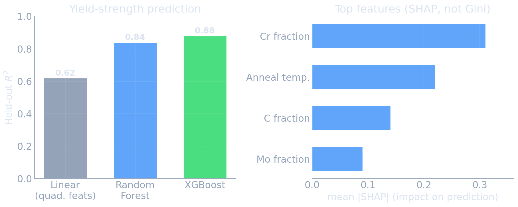
Typical pattern: tree ensembles add 10–20 points of \(R^2\) over linear models at essentially no engineering cost.

• This is the “why you just sat through 40 slides” slide — a concrete, representative materials result. The jump from 0.62 → 0.88 with no feature engineering, no scaling, default-ish hyperparameters is the entire value proposition in one number.
• Note the SHAP framing (not raw impurity) — practice what the importance slide preached; reinforce by saying “I deliberately reported SHAP here, not Gini importance.”
• Honest caveats to state: numbers are illustrative-typical; held-out split must respect alloy families (no near-duplicate leakage across train/test) or R² is optimistic — connect to the OOB/CV assumptions and the Unit 7 exchangeability caveat. Good students will ask; pre-empt it.

Which model when — a decision guide

• First baseline, any tabular problem: Random Forest (robust, OOB, importances, ~no tuning).
• Best tabular accuracy, typical materials data: CatBoost first (categorical-heavy, near-optimal at defaults); XGBoost as the general-purpose workhorse; LightGBM if \(N>10^6\).
• Small data (\(\lesssim 10\)k): also benchmark TabPFN.
• Images / spectra / sequences / graphs: neural networks (Units 9–13), not trees.
• Always: respect the train/val/test split, early-stop boosting, report honest (permutation/SHAP) importances.

• The capstone “what do I actually type” slide — students should photograph this and the tuning recipe. It is the operational distillation of the whole unit.
• Re-emphasize the workflow discipline in the last bullet: the split integrity and honest-importance rules are where real projects fail, not the model choice. Tie back to Unit 7 (data leakage = broken exchangeability) and forward to Unit 14 (honest reporting).
• One sentence on the applied-course dependency: ML-PC Units 7–8 and Materials Genomics assume this decision guide as background — students who skip it will be lost there. Frame mastery here as load-bearing for the rest of the track.

Bias–variance summary across this unit

Method	Bias	Variance	Mechanism
Single deep tree	low	high	flexible greedy partition
Bagging	low	reduced	average bootstrap trees
Random Forest	low	strongly reduced	+ decorrelate via feature subsets
Gradient Boosting	reduced	medium	sequentially fit residuals
XGBoost (regularized)	reduced	controlled	+ leaf penalty, shrinkage, early stop

• This table is the unit’s mental model in one frame — and it should map exactly onto the two-arrow diagram you put on the board in slide 3. Walk each row pointing at “↓Var” or “↓Bias.” If a student can reconstruct this table from the two arrows, the unit succeeded.
• Use it as the active-recall checkpoint: cover the last two columns, name a method, have the room supply bias/variance/mechanism. 60 seconds, high retention.
• Transition to wrap-up: every method here was one move on the trade-off Units 6–7 set up — the course is one coherent argument, not a list of algorithms.

Unit summary

• A decision tree is a fast, interpretable, piecewise-constant partitioner — and a low-bias, high-variance learner.
• Bagging / Random Forest kill variance by averaging decorrelated trees; the correlation \(\rho\) sets the floor, which is why RF subsamples features.
• Gradient boosting is gradient descent in function space; it kills bias by sequentially fitting pseudo-residuals, controlled by shrinkage + early stopping.
• Gradient-boosted trees are the 2026 tabular default — CatBoost for the categorical-heavy materials data here, XGBoost as the general workhorse, LightGBM at large \(N\); trees beat NNs on tabular for concrete, understood reasons (TabPFN the emerging exception).
• Interpret with permutation importance / TreeSHAP, never raw impurity in a paper.

• Deliver three sentences they must leave with: (1) tabular materials problem → gradient boosting first, NN only if data shape demands it; (2) RF reduces variance, boosting reduces bias — name the floor (ρσ²) and the cure (shrinkage + early stopping); (3) report honest importances (permutation/SHAP), not Gini.
• Close the course-level arc: Units 6–8 are one argument — the loss landscape (6), the probabilistic meaning of the loss (7), and the models that best navigate the bias–variance trade-off on real tabular data (8). Then point at the Unit 9 reading: we now leave tabular for learned representations.

Common pitfalls and best practices

• Data leakage: target-derived features, or train/test split that ignores alloy/batch grouping → inflated scores.
• Over-trusting impurity importance as if it were causal — it is biased and not causal.
• No early stopping on boosting → silent overfitting.
• Forgetting trees ≠ extrapolation: predictions are flat outside the training range — dangerous for materials discovery in new composition regions.
• Over-tuning: defaults + early stopping beat a frantic grid search more often than students expect.

• This slide is deliberately a list of the specific ways the materials cohort’s projects will actually fail — it is worth more than another algorithm. Dwell on the extrapolation point: tree ensembles predict a constant outside the training hull, so using them to discover alloys in unexplored composition space gives confident, flat, wrong answers. Pair with epistemic-uncertainty/conformal from Unit 7 as the mitigation.
• Grouped-leakage is the second killer: random row splits on data with near-duplicate alloy families leak information and inflate R²; split by group. This is the single most common reason a materials ML result fails to reproduce.
• End on the over-tuning reassurance — it lowers anxiety and is true: sensible defaults + early stopping + honest evaluation beats hyperparameter panic.

Lecture-essential vs exercise content split

• Lecture: tree mechanics + impurity, the bagging variance formula and the \(\rho\) ceiling, RF decorrelation + OOB, gradient boosting as functional gradient descent, regularization, model choice.
• Exercise: build a regression tree from scratch; RF vs single tree on alloy data with OOB; XGBoost with early stopping + a learning-curve sweep; permutation vs TreeSHAP importances; RF/XGBoost baseline on the alloy regression task.

• Set expectations: the written exam tests concepts and the two derivations (bagging variance formula, functional-gradient view) and model-choice reasoning; the coding exercise tests the workflow (early stopping, honest importances, the decision guide).
• Stress the cross-track dependency again: ML-PC Units 7–8 use RF/XGBoost as the assumed tabular workhorse and expect the exercise to have been done. Skipping it has a concrete downstream cost — frame it as non-optional.

Exam-aligned summary: must-know statements

1. A decision tree partitions feature space into axis-aligned boxes via greedy impurity reduction.
2. Regression impurity = within-node variance; classification = Gini or entropy (≈ equivalent).
3. A single deep tree is low-bias, high-variance, and unstable.
4. Bagging averages bootstrap trees: \(\mathrm{Var}=\rho\sigma^2+\frac{1-\rho}{B}\sigma^2\) → floor at \(\rho\sigma^2\).
5. Random forest lowers \(\rho\) by random feature subsets per split — that is why it beats plain bagging.
6. OOB error is a near-free generalization estimate from the ~37% unused points.
7. Impurity importance is biased; use permutation or TreeSHAP, and never claim causality.
8. Boosting reduces bias by sequentially fitting pseudo-residuals (= negative loss gradient).
9. Gradient boosting = gradient descent in function space; \(\eta\) is its learning rate.
10. Boosting overfits without early stopping; small \(\eta\) + many trees + early stop is the recipe.
11. XGBoost adds a 2nd-order objective + leaf penalties (general-purpose workhorse); CatBoost (ordered target statistics + ordered boosting) is the near-zero-tuning default for categorical-heavy materials data.
12. On tabular data trees usually beat NNs (uninformative features, non-smooth targets, axis meaning); TabPFN is the emerging small-data exception.

• This is the revision sheet — run it as cold-call active recall: read the statement, the room supplies the justification. Statements 4, 5, 8, 9 are the conceptual spine (the two derivations); weight them heaviest in review and on the exam.
• Statement 7 is the one with real-world scientific stakes (it prevents a publishable error); statement 12 is the one that changes their default modeling choice for the rest of the track. Flag both as “remember this even if you forget the formulas.”
• Close: this list is exactly the Learning Outcomes slide, now assessable — the unit delivered its contract. Point to the Unit 9 reading and the transition from tabular models to learned representations.

Continue

• ← Previous: Unit 07 — Probabilistic View of Learning; Noise; Conformal Prediction
• → Next: Unit 09 — Latent Spaces & Advanced Representation Learning
• All courses

References + reading assignment for next unit

• Required reading before Unit 9:
  • Murphy: Ch. 28 (representation learning) — skim the SSL chapter intro.
  • Bishop: Ch. 12.1–12.3 (continuous latent variable models, PCA revisited).
• Optional depth:
  • Hastie, Tibshirani & Friedman, ESL Ch. 9–10 & 15 (trees, boosting, random forests).
  • Grinsztajn et al. 2022 — why trees beat deep learning on tabular data.
• Next unit: Latent Spaces & Advanced Representation Learning — t-SNE, UMAP, contrastive and self-supervised methods.

Breiman, Leo. 1996. “Bagging Predictors.” Machine Learning 24 (2): 123–40.

Breiman, Leo. 2001. “Random Forests.” Machine Learning 45 (1): 5–32.

Chen, Tianqi, and Carlos Guestrin. 2016. “XGBoost: A Scalable Tree Boosting System.” Proceedings of the 22nd ACM SIGKDD International Conference on Knowledge Discovery and Data Mining.

Freund, Yoav, and Robert E. Schapire. 1997. “A Decision-Theoretic Generalization of on-Line Learning and an Application to Boosting.” Journal of Computer and System Sciences 55 (1): 119–39.

Friedman, Jerome H. 2001. “Greedy Function Approximation: A Gradient Boosting Machine.” Annals of Statistics 29 (5): 1189–232.

Geurts, Pierre, Damien Ernst, and Louis Wehenkel. 2006. “Extremely Randomized Trees.” Machine Learning 63 (1): 3–42.

Grinsztajn, Léo, Edouard Oyallon, and Gaël Varoquaux. 2022. “Why Do Tree-Based Models Still Outperform Deep Learning on Tabular Data?” Advances in Neural Information Processing Systems (NeurIPS), Datasets and Benchmarks Track. https://arxiv.org/pdf/2207.08815.

Hollmann, Noah, Samuel Müller, Katharina Eggensperger, and Frank Hutter. 2023. “TabPFN: A Transformer That Solves Small Tabular Classification Problems in a Second.” International Conference on Learning Representations (ICLR). https://arxiv.org/abs/2207.01848.

Ke, Guolin, Qi Meng, Thomas Finley, et al. 2017. “LightGBM: A Highly Efficient Gradient Boosting Decision Tree.” Advances in Neural Information Processing Systems (NeurIPS).

Lundberg, Scott M., Gabriel Erion, Hugh Chen, et al. 2020. “From Local Explanations to Global Understanding with Explainable AI for Trees.” Nature Machine Intelligence 2 (1): 56–67.

Lundberg, Scott M., and Su-In Lee. 2017. “A Unified Approach to Interpreting Model Predictions.” Advances in Neural Information Processing Systems (NeurIPS).

Prokhorenkova, Liudmila, Gleb Gusev, Aleksandr Vorobev, Anna Veronika Dorogush, and Andrey Gulin. 2018. “CatBoost: Unbiased Boosting with Categorical Features.” Advances in Neural Information Processing Systems (NeurIPS).

Example Notebook

Week 8: Tree Ensembles — RF & XGBoost on alloy regression

Open rendered notebook →