Mathematical Foundations of AI & ML
Unit 14: Explainability, Limits, and Trust

Prof. Dr. Philipp Pelz

FAU Erlangen-Nürnberg

Title + Unit 14 positioning

• The final lecture of Mathematical Foundations of AI & ML.
• From physics-informed learning (Unit 13) to the question: can we trust our models?
• We synthesize the entire 14-unit arc into a coherent methodology for trustworthy ML.

• This is the last lecture — open by naming that explicitly and setting the tone: today is not new machinery, it is the question every previous unit was secretly building toward. “We spent 13 units making models work; today we ask whether we are allowed to believe them.”
• The one sentence to land hard: a model that predicts correctly but cannot be interrogated is, for an engineer, not finished — it is a liability waiting for an audit. Say it before any content; it is the moral of the whole unit.
• Materials anchor for this cohort: frame it as the difference between “the network says this weld will hold” and “the network says this weld will hold because of these three measured features, and here is how confident it is.” Only the second is something you sign your name under.
• Misconception to preempt now: students think explainability is a soft, optional topic bolted on at the end. Reframe immediately — it is a hard mathematical and regulatory constraint (EU AI Act, falsifiability) that we will treat with the same rigor as the GP posterior in Unit 12.
• Transition: “Here is exactly what you will be able to do by minute 90 —” → learning outcomes.

Learning outcomes for Unit 14

By the end of this lecture, students can:

• explain why explainability is a scientific and industrial mandate,
• distinguish semantic structures (synonyms, taxonomies, ontologies),
• perform and interpret perturbation-based sensitivity analysis,
• assess where ML adds value in causal process chains and where it fails.

• Don’t read the list — turn it into a contract. Each outcome maps to one block of the 90 minutes and to one of the “10 must-know statements” at the end; tell them the exam surface is fixed and visible, exactly as you did in Units 7 and 12.
• Flag the two outcomes students will be examined on most directly: (3) perform and interpret perturbation sensitivity — a numerical/derivation question — and (1) why explainability is a mandate — the conceptual essay question. The semantic-structures outcome (2) is recall-level; the causal outcome (4) is the judgement question that separates top marks.
• Calibrate rigor up front: this unit is conceptually broad but mathematically light compared to 12. The deliverable is judgement — “can you say where a model should and should not be trusted, and defend it” — not a theorem. Set that expectation so they don’t wait for heavy algebra that isn’t coming.
• Transition: “Start with the hardest question — why can’t we just ship the accurate black box?”

Why explainability is non-negotiable

• Science demands understanding, not just prediction — a model that cannot be questioned cannot be falsified.
• Industry demands accountability — engineers must justify decisions to stakeholders.
• Regulation demands transparency — EU AI Act requires explanations for high-risk AI systems.
• Explainability is not optional — it is a prerequisite for deploying ML in engineering.

• Three audiences, three independent forcing functions — make clear that any one of them is sufficient to kill an unexplained model; you do not need all three. Science alone (falsifiability) is enough for the researchers in the room; regulation alone is enough for anyone who will ever ship.
• The science bullet is the deep one — connect it to Popper explicitly (the next-but-one slide formalizes this): a prediction you cannot question is a prediction you cannot test, and an untestable claim is not science. This is the intellectual spine of the unit; the regulatory and industrial points are the practical teeth.
• Concrete EU AI Act hook for a German engineering cohort: high-risk AI (which includes safety-relevant industrial QC) carries a legal right to explanation. This is not aspirational — it is in force and it constrains what they are allowed to deploy after they graduate. Make it personal: “this will be your problem, not a slide’s.”
• Misconception to preempt: “accuracy buys trust.” No — accuracy on the test set buys nothing with a regulator or a falsification-minded scientist if the mechanism is opaque. Decouple “is it right” from “can we justify it”; the rest of the unit lives in that gap.
• Transition: “So what exactly is the obstacle? Name the enemy —” → the black-box problem.

The black-box problem

• Deep neural networks achieve remarkable accuracy but offer no explanation for individual predictions.
• A model predicting “this alloy will fail” without explaining why is unacceptable for safety-critical decisions.
• Engineers need to know which factors drive the prediction and how confident the model is.
• The black-box problem motivates the entire field of explainable AI (XAI) (Neuer et al. 2024).

• Define “black box” precisely so it isn’t a slur: it is a model whose input–output map is accurate but whose internal decision path is not expressible in terms a domain expert can check against physics. A deep net is a black box; a 4-term linear model on interpretable features is not. The property is legibility of the mechanism, not complexity per se.
• The “which factors / how confident” pairing on the third bullet is the thesis of the entire unit in one line: explainability (which factors — §E3/SHAP) and uncertainty (how confident — the Unit 12 callback). Say explicitly that today completes the pair we started in 12; trust = explanation + calibrated confidence, never one alone.
• Materials example to make it visceral: an alloy-failure classifier at 97% accuracy that, on inspection, keyed on a furnace-ID artifact correlated with one supplier. Same accuracy number, worthless model — and you only catch it by opening the box. This previews the confounding/causality section; plant it here.
• Honest nuance for the strong students: “black box” is relative to the questioner. Mechanistic interpretability (later in §8) is the research bet that even deep nets are not intrinsically opaque — we just lacked the tools. Foreshadow, don’t resolve.
• Transition: “If opacity is the disease, the first cure is a precise vocabulary — interpretability is not the same thing as explainability.”

Explainability vs interpretability

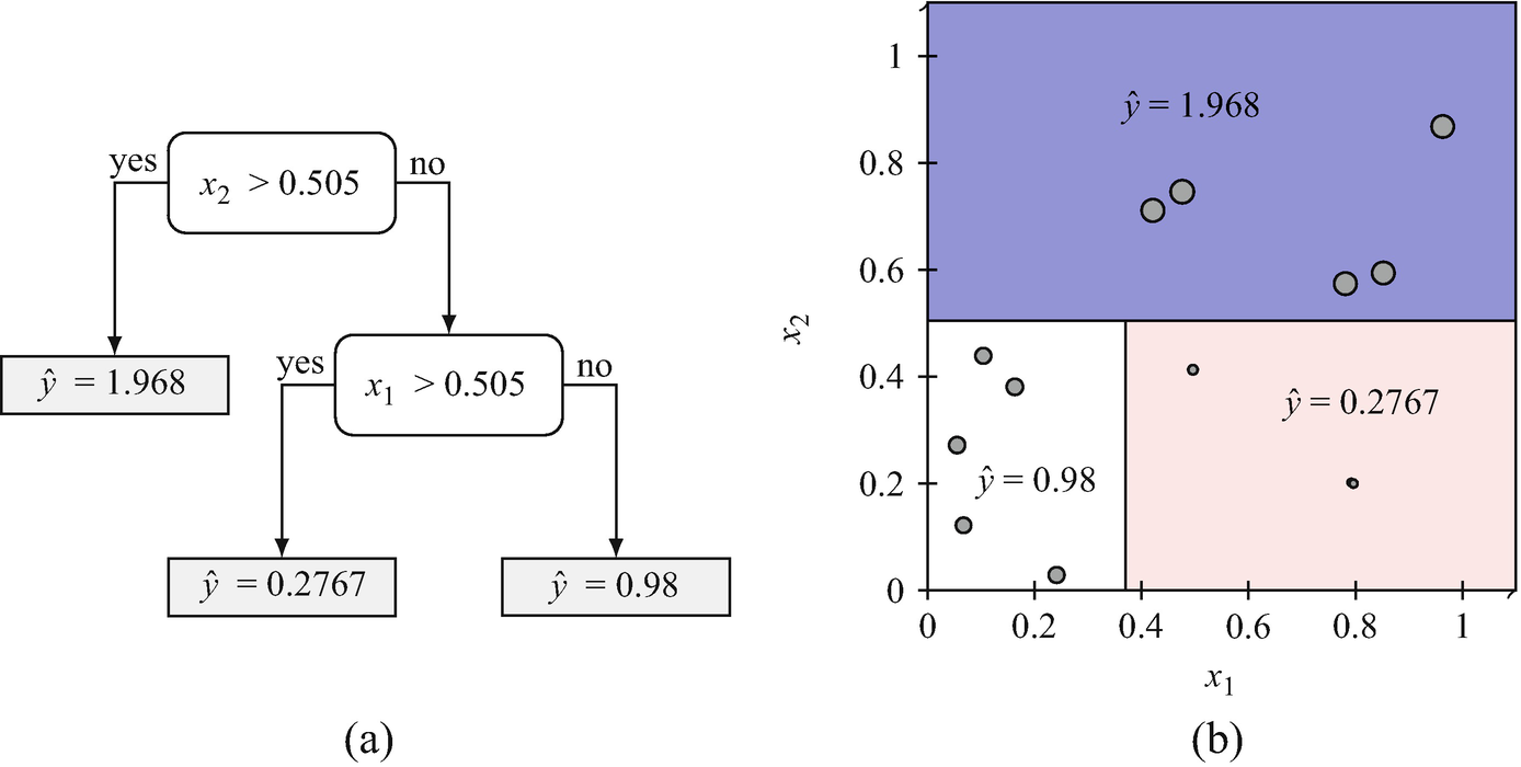
Interpretability

• The model itself is transparent and understandable.
• Examples: linear regression, decision trees, small rule sets.

Explainability

• Post-hoc methods that reveal the reasoning of complex models.
• Examples: SHAP values, sensitivity analysis, attention visualization.

• Trade-off: interpretable models may be less accurate; explainability adds complexity to accurate models.

A three-leaf decision tree and the corresponding partition of input space — an inherently interpretable model (McClarren 2021)

• This is the single most important distinction in the unit — make students write the two definitions verbatim. Interpretability = the model is transparent by construction (you can read the mechanism off the parameters). Explainability = the model is opaque, so you attach a separate post-hoc method that approximates its reasoning. One is a property of the model; the other is a tool you bolt on.
• The figure is the canonical interpretable model: trace the tree to its axis-aligned partition and say “the explanation is the model — there is nothing post-hoc here.” Contrast immediately with the deep net from the previous slide, where the explanation is a second artifact that can itself be wrong.
• Land the trade-off bullet as the central engineering tension of the unit, the analogue of bias–variance: a glass-box model you fully trust but that may underfit, versus an accurate black box plus an approximate explanation you must also validate. There is no free lunch — choosing is an engineering decision, not a default.
• Misconception to kill hard: “SHAP makes a neural net interpretable.” It does not — it makes it explainable. The net is still a black box; SHAP is a faithful-only-approximately story about it that can mislead (we prove this in §8). Keep the words separate all unit; sloppy vocabulary here causes wrong conclusions later.
• Exam hook: “name one interpretable and one explainable method and state which property each has” is the cleanest possible definition question — flag it.
• Transition: “Transparent to whom? Different people need different explanations —” → who needs explanations.

Who needs explanations?

• Scientists: full understanding (all levels) — to build knowledge.
• Engineers: process and prediction level — to make decisions.
• Regulators: data provenance and prediction justification — to ensure compliance.
• Operators: actionable recommendations — to adjust process parameters.
• Different audiences need different types and depths of explanation.

• This slide is the seed of the E1–E6 framework — say so explicitly: “hold this list; in 20 minutes each audience maps to specific levels.” It turns a vague ‘explainability is good’ into an engineering spec: who is the recipient, what decision do they make, what depth do they need.
• The operational point students miss: an explanation is not true or false in the abstract — it is fit for a recipient and a decision. A SHAP plot is a perfect explanation for a data scientist and a useless one for a furnace operator who needs “raise temperature by 20 °C.” Same model, same prediction, different correct explanation.
• Materials cohort anchor: walk the four audiences through one scenario — a sintering-defect predictor. Scientist wants the structure–property mechanism; engineer wants which parameters to tune; regulator wants data provenance + per-part justification; operator wants the actionable setpoint. One model, four explanations.
• Misconception to preempt: “more detail is always better.” No — over-explaining to an operator buries the action; under-explaining to a regulator fails the audit. Matching depth is the skill, not maximizing it.
• Transition: “What does it cost when you get this wrong — when the explanation is missing entirely?”

The cost of unexplainability

• Rejected by regulators (cannot approve what cannot be explained).
• Distrusted by domain experts (they will use their own judgment instead).
• Impossible to debug (when predictions fail, no path to diagnosis).
• Liability risk (who is responsible when an unexplained model causes harm?).

• Frame these as four independent failure modes, not a rhetorical list — each one alone sinks a deployment. The point is that the costs are not hypothetical or distant; they are the four ways real industrial ML projects die after the demo works.
• Spend most time on “impossible to debug” — it is the one engineers feel viscerally. When an opaque model fails in production you have no gradient to follow back to a cause; you are reduced to retraining and praying. An explainable model fails informatively. This is the day-to-day, not-headline cost they will actually live with.
• The liability bullet is the one that wakes the room: ask “if your unexplained model green-lights a part that then fails catastrophically, who signs the incident report — you, your supervisor, or the network?” There is no good answer, which is exactly the point and why regulators force the issue.
• Tie back: the “distrusted by experts” bullet is why interpretable models (previous slide) sometimes win despite lower accuracy — a model the expert overrides has zero deployed value regardless of its test metrics. Effective accuracy = model accuracy × probability the expert actually uses it.
• Transition: “These are practical costs. But there is a deeper, almost philosophical reason — explainability is what makes ML science rather than alchemy.”

Explainability as scientific method

• Science progresses by proposing models, deriving predictions, and testing them.
• A model that cannot be questioned cannot be falsified — it fails Popper’s criterion.
• ML models that only predict without explanation are tools, not science.
• Making ML explainable elevates it to a scientific methodology.

• This is the intellectual high point of the framing — slow down and make the Popper argument carefully. A model that only emits predictions and cannot say why makes no risky, falsifiable claim about mechanism; it is an oracle, not a theory. Oracles can be accurate and still be unscientific.
• Sharpen the “tools vs science” line: a pure black-box predictor is a sophisticated lookup table — useful engineering, but it adds no understanding, so it cannot be wrong in an interesting way and cannot be improved by being refuted. Explanation is what gives the model a falsifiable surface.
• Connect forward to §10 (deductive reasoning with ontologies): that slide is the concrete machine for this philosophy — an explanation states “feature X drives the prediction via mechanism M,” and the ontology lets you test that against known physics. Falsifiability becomes an automated consistency check, not a slogan.
• Pre-empt the cynical student (“isn’t this just philosophy?”): no — it is the operational reason the EU AI Act and journal reviewers both demand explanations. Falsifiability is the shared root of the scientific mandate and the regulatory one; that is why the two pressures point the same way.
• Transition: “With the why settled, place today inside the whole course — every unit was a step toward this question.” → course context.

Course context

• Every unit has built toward this moment:
  • Loss minimization (Unit 1): what does the model optimize?
  • Generalization (Unit 8): does it work on new data?
  • Uncertainty (Unit 12): how confident is it?
  • Physics (Unit 13): does it respect known laws?
  • Explainability (Unit 14): can we understand and trust it?

• Deliver this as a payoff slide, not a recap — the students built each of these tools without seeing the destination; now show that the whole course was an arc with this unit as the keystone. The emotional beat is “everything you learned was load-bearing for this question.”
• Hit the four named callbacks deliberately, because each returns concretely later today: loss minimization → “what does it optimize” is the E4 model-level question; generalization → underlies the data-manifold-limits slide; uncertainty (Unit 12) → is literally half of “trust” and recurs in OOD detection; physics (Unit 13) → is the falsifiability test in the ontology slide. Tell them to expect these returns.
• The unifying sentence to say aloud and reuse all lecture: trust = it optimizes the right thing (loss) + it generalizes + it knows what it doesn’t know (uncertainty) + it respects known law (physics) + we can interrogate why (explainability). Five conditions; today supplies the fifth and shows it binds the other four.
• Misconception to preempt: that explainability is a separate sub-field tacked on. Reframe — it is the integration layer; without it the other four are private virtues the model cannot demonstrate to anyone who matters.
• Transition: “Concretely, here is how the 90 minutes are spent —” → roadmap.

Roadmap of today’s 90 min

• 10–25 min: Semantic structures — digitizing meaning.
• 25–40 min: Six levels of explainability (E1–E6).
• 40–55 min: Sensitivity analysis — perturbation and beyond.
• 55–65 min: Causality in process chains.
• 65–75 min: Data manifold limits and trust.
• 75–87 min: Course retrospective — the 14-unit arc.

• This is your pace contract and your recovery tool — the two checkpoint slides (semantic structures, causality) are deliberate buffers. If you are behind, compress the semantic-structures block (it is recall-level) and protect the sensitivity-analysis block, which carries the only examinable derivation in the unit.
• Tell students where the exam weight sits so they listen with the right intensity: the 40–55 min sensitivity block and the 65–75 min trust/limits block are the high-yield core; semantics (10–25) is foundational vocabulary; the retrospective (75–87) is exam-prep scaffolding, not new content.
• Set expectation on texture: the first half is conceptual/vocabulary-heavy and moves fast; the middle is the one place we slow down and compute (the sensitivity formula); the end zooms back out. Warn them so the pace changes feel intentional, not erratic.
• Transition: “We start with a problem that sounds linguistic but is deeply mathematical — how do you put meaning into a model that only eats numbers?”

Digitizing meaning: the challenge

• ML models operate on numbers (tensors, vectors, matrices).
• Domain knowledge is encoded in language and relationships.
• Bridging this gap requires semantic structures that formalize meaning.
• Without semantic structures, models cannot be grounded in domain understanding (Neuer et al. 2024).

• Frame the gap precisely: a model sees a column of floats; the engineer sees “yield strength of a heat-treated alloy.” Nothing in the tensor records that the column means that, that it has units, or that it relates causally to other columns. Explainability requires re-attaching that meaning the featurization stripped off.
• The key reframe for this block: semantic structures (synonyms → taxonomies → ontologies) are not NLP or knowledge-graph trivia — they are the scaffold that lets every later explanation (E1–E6, the falsifiability check, causal chains) be stated in domain terms a scientist can validate. Without them an explanation is just “feature 7 mattered,” which is unfalsifiable.
• Materials anchor: the same physical property arrives from three labs as “Rp0.2”, “yield strength”, “σ_y” in two unit systems. To the model these are unrelated dimensions. The cost of not digitizing meaning is double-counted features and explanations that name aliases instead of physics.
• Misconception to preempt: students think this is solved by “just clean your data.” It is not a cleaning step — it is an explicit, reusable model of the domain (next three slides build it up in increasing power). Cleaning is ad hoc and per-dataset; a semantic structure is portable and inspectable.
• Transition: “Start at the simplest rung — naming the same thing the same way.” → synonyms and controlled vocabularies.

Synonyms and controlled vocabularies

• Different terms for the same concept: “yield strength” = “elastic limit” = “\(R_e\)”.
• Controlled vocabulary: a standardized list of terms with defined meanings.
• Without synonym resolution, models may treat the same property as two separate features.
• First step in any data integration pipeline.

Semantic tools ordered by increasing complexity (Neuer et al. 2024)

• Use the figure as the spine of the whole semantics block: synonyms → controlled vocabulary → taxonomy → ontology is a ladder of increasing expressive power and increasing cost to build. Tell them we climb it over the next four slides; each rung buys a stronger kind of explanation.
• Make the synonym example concrete and physical: “yield strength = elastic limit = \(R_e\)” are not just spellings — different labs, standards (DIN vs ASTM), and eras. A controlled vocabulary is the social/engineering act of forcing one canonical name; the payoff is that an explanation can finally say “driven by yield strength” instead of “driven by feature_12 and feature_31,” which the model wrongly treated as independent.
• The single sentence to land: unresolved synonyms don’t just waste columns — they split one cause across two features, so feature-importance and SHAP attributions get halved and the explanation becomes literally wrong. This is the hook for the §8 sensitivity caveats; plant it now.
• Misconception to preempt: “the model will learn they’re the same.” Only if it has enough data to discover the redundancy — and it still cannot tell you they were synonyms. You pay in sample efficiency and in explanation fidelity. Cheap to fix here, expensive to detect later.
• Transition: “Once names are canonical, the next rung adds hierarchy — taxonomies.” → taxonomies.

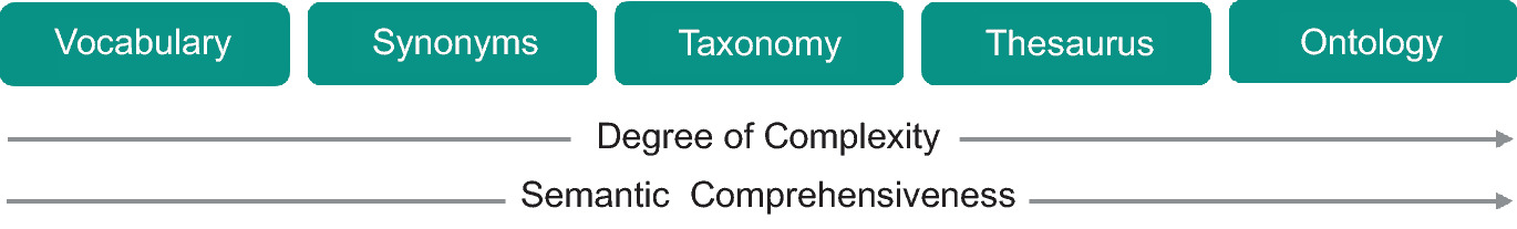
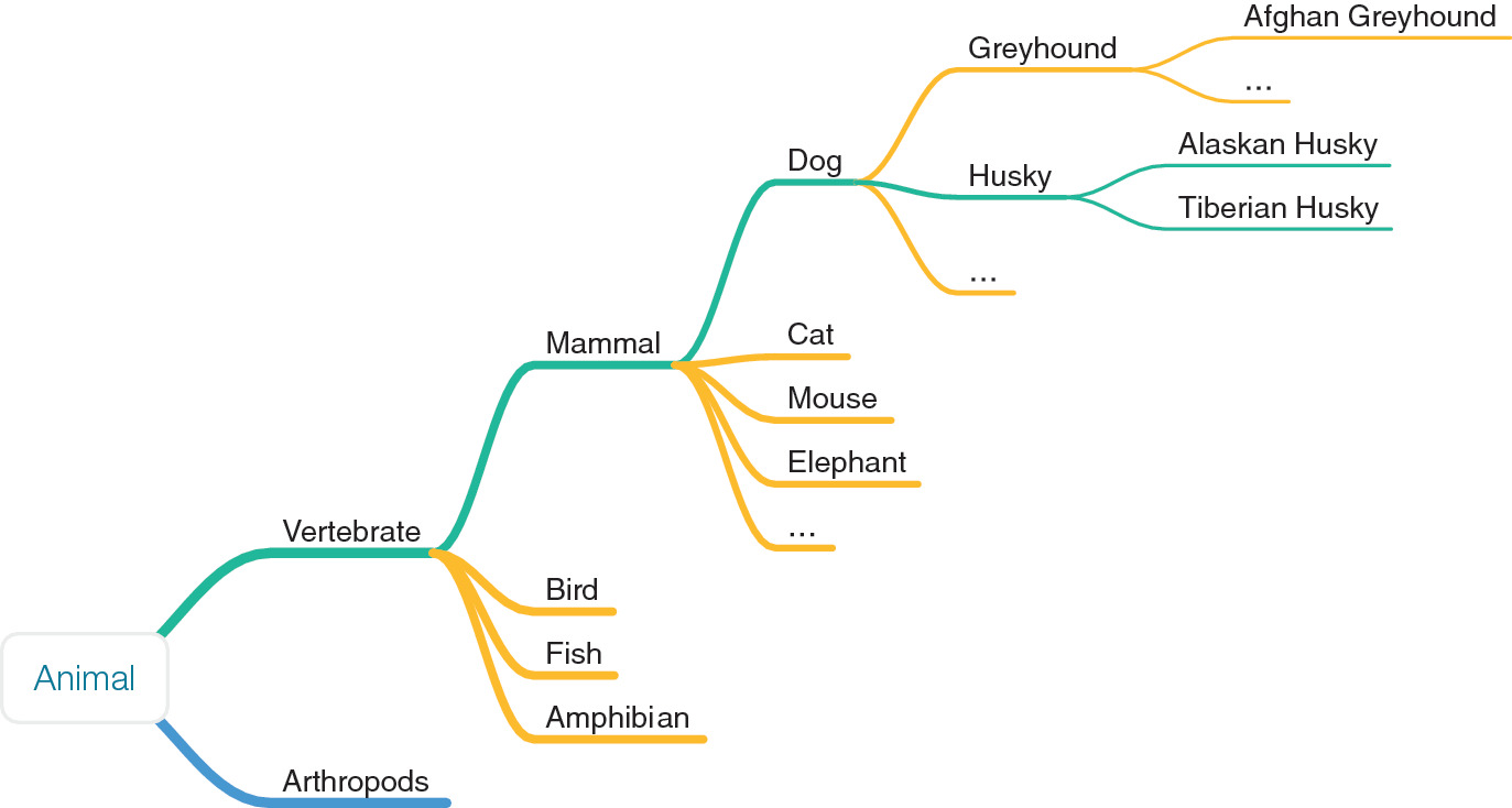
Taxonomies: hierarchical classification

• Organize concepts in parent-child hierarchies:
  • Material > Metal > Steel > Stainless Steel > 316L.
• Taxonomies enable inheritance: properties of “Metal” apply to all sub-categories.
• They structure domain knowledge and guide feature selection.

Example taxonomy from biology: vertebrates and arthropods (Neuer et al. 2024)

• The one new idea over synonyms is inheritance — say the word and make it do work: properties asserted at “Metal” hold for “316L” without restating them. This is what lets an explanation generalize (“this failure mode is a metal phenomenon, not specific to 316L”) instead of staying instance-bound.
• The biology figure is a deliberate neutral example so the structure is obvious before the materials transfer; walk one path root-to-leaf, then immediately re-instantiate it in their domain: Material > Metal > Steel > Stainless > 316L. Do the re-instantiation aloud — that transfer is the learning objective, not the biology.
• Pedagogical payoff to state: a taxonomy gives feature selection a prior — if “grain size” matters for “Steel,” it is a candidate for every steel subclass. This is the seed of the §4 “ontologies for feature engineering” slide and connects to the inductive-bias theme of Unit 8.
• Misconception to preempt: a taxonomy is not a clustering result. Clustering is discovered bottom-up from data and can be wrong; a taxonomy is asserted top-down from domain knowledge and is the thing you check the data against. Different epistemic status — one is a hypothesis, the other is the reference.
• Honest limit / transition: taxonomies only express is-a. Real domain knowledge has affects, measured-in, determines — arbitrary relations. “For that we need the top rung —” → ontologies.

Ontologies: structured knowledge graphs

• An ontology defines concepts, relationships, and constraints:
  • “Alloy hasProperty tensileStrength”
  • “tensileStrength measuredIn MPa”
  • “grainSize affects yieldStrength”
• Richer than taxonomies: capture arbitrary relationships, not just hierarchies.

• Define the triple precisely — subject–predicate–object — and read the three examples as sentences: “alloy has-property tensile-strength,” “tensile-strength measured-in MPa,” “grain-size affects yield-strength.” The third is the one that matters: it encodes a physical mechanism, not just structure. That is the qualitative jump from taxonomy.
• The sentence to land: an ontology turns domain knowledge into machine-checkable statements. “grain-size affects yield-strength” is a falsifiable claim the model’s explanation must be consistent with — this is the literal mechanism behind the §10 deductive-reasoning slide and the falsifiability promise from §2. Foreshadow that explicitly: “remember this triple; in 30 minutes we audit a model against it.”
• Materials anchor: the three core relations they will reuse all course — determines, affects, measured-in — line up with the composition→processing→microstructure→properties chain that recurs in the next slide and again in the causality section. Tell them this is the same backbone, formalized.
• Misconception to preempt: an ontology is not a database schema. A schema says what can be stored; an ontology says what is true and entailed (inheritance + relations support inference). Confusing the two makes the §10 consistency check look like mere validation rather than reasoning.
• Transition: “Why should an ML engineer, not a knowledge-engineer, care? Three concrete payoffs —” → why ontologies matter for ML.

Why ontologies matter for ML

• Enable deductive reasoning: if the model’s prediction violates a known ontological relationship, flag it.
• Guide feature engineering: ontological relationships suggest which features to include.
• Support consistency checking: predictions must be consistent with domain constraints.
• Provide a framework for communicating model behavior to domain experts.

• Four payoffs, but they are not equal — flag the first (deductive reasoning / consistency) as the load-bearing one for this unit; the other three are valuable but the falsifiability check is the one that connects ontologies to the scientific-method argument from §2 and gets its own slide in §10.
• Make “consistency checking” concrete with a number: if the ontology says grain-size affects yield-strength but the trained model assigns it ~0 importance, that is not noise — it is a contradiction that flags either a data problem (no grain-size variation in the sample) or a broken model. The ontology gave you a unit test for the explanation.
• The feature-engineering payoff is the bridge to Unit 13: ontological relations are encoded physics knowledge. Tell them an ontology is the discrete, symbolic cousin of a physics-informed loss term — both inject prior structure, one as hard logical constraints, the other as a soft penalty.
• Misconception to preempt: “this only helps if the ontology is complete/perfect.” No — even a partial ontology catches contradictions in the relations it does assert. It is a sound but incomplete check (it never wrongly flags a true model; it just may miss some bad ones). Frame it as a safety net, not a proof system.
• Transition: “Take the most useful payoff — feature engineering — and see it on a real process ontology.” → ontologies for feature engineering.

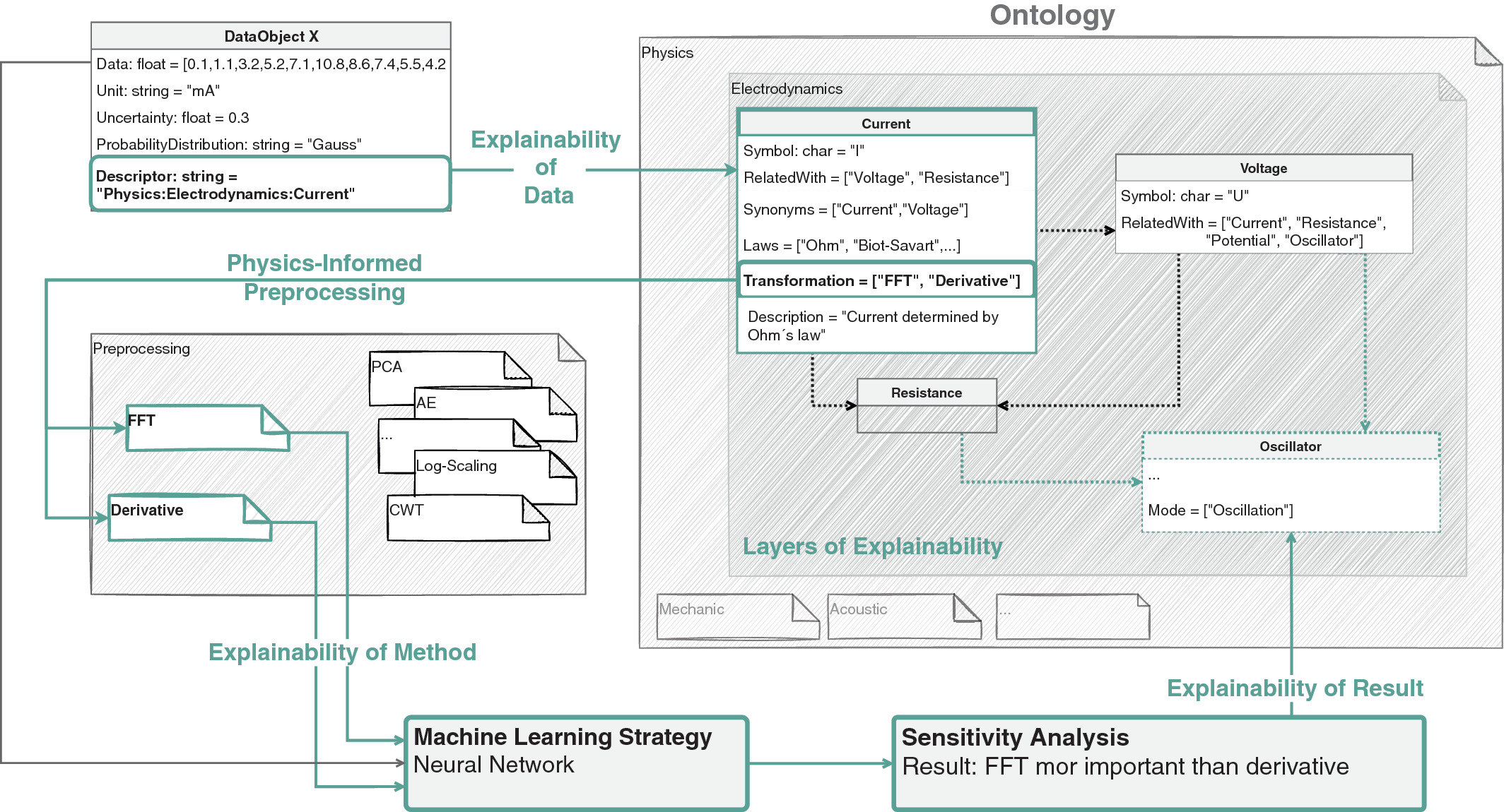
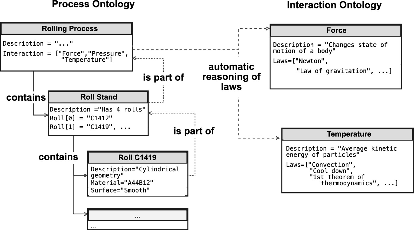
Ontologies for feature engineering

• Ontological relationships encode domain knowledge about what matters:
  • “Composition determines phase” → include composition features.
  • “Processing affects microstructure” → include processing parameters.
• This connects to Unit 13 (physics-informed learning): ontologies formalize the physics knowledge.

Process ontology combining process descriptions with physical interactions (Neuer et al. 2024)

• This slide closes the semantics ladder by making it actionable: the ontology doesn’t just describe — it prescribes which columns belong in your feature matrix. Read the two rules off the figure as engineering instructions: “composition determines phase” → put composition features in; “processing affects microstructure” → include processing parameters.
• The explicit Unit 13 callback is the one to dwell on — say it slowly: an ontology is physics knowledge in symbolic form; a PINN is the same knowledge in differentiable form. Two encodings of one prior. This is the conceptual bridge that makes the whole “trust” cluster (Units 13–14) coherent rather than two separate topics.
• The deep point for strong students: ontology-guided feature selection is principled inductive bias (Unit 8) — you restrict the hypothesis space using domain truth rather than a generic regularizer. That is why it improves generalization, not just interpretability. Same mechanism as L2, better-informed prior.
• Misconception to preempt: “the model should discover relevant features itself.” It can, given enough data — but ontology-guided selection gets there with far fewer samples and yields an explanation already phrased in domain relations, so it is auditable by construction. Trade data for prior knowledge; in materials, data is the scarce resource.
• Transition: “Make this fully concrete with the canonical materials ontology — the causal chain you will see in every applied unit.” → materials ontology example.

Materials ontology example

• Causal chain: Composition \(\) Processing \(\) Microstructure \(\) Properties.
• This is a process ontology — each arrow represents a physical mechanism.
• Models should respect this chain: predicting properties from composition is valid; the reverse is an ill-posed inverse problem.

• This is the slide of the semantics block — the composition→processing→microstructure→properties chain is the single most reused object in the entire applied curriculum. Tell them to memorize it; it returns verbatim in the causality section today and underlies Units 9, 11, 13.
• Land the forward-vs-inverse asymmetry hard, because it is both a physics fact and an exam-grade insight: forward (composition → properties) is well-posed — one cause, one effect. Inverse (properties → composition) is ill-posed — many compositions yield the same property, so the map is one-to-many and a naive regressor will average across modes and output a physically meaningless blend. Connect to generative models (Unit 11): the right way to invert is to model the full conditional distribution, not predict a point.
• Each arrow is a physical mechanism, not a correlation — say this explicitly; it is the setup for the §9 causality slides where we contrast this with spurious correlations. The ontology arrow direction is knowledge we impose, not something the data can tell us.
• Misconception to preempt: “more layers / more data fixes the inverse problem.” No — ill-posedness is a property of the physics, not the model. No amount of capacity makes a one-to-many map a function. This kills the common student instinct that any mapping is learnable with enough net.
• Transition: “Quick check that the semantics block landed —” → checkpoint.

Checkpoint: semantic structures

• Question: Your model uses “hardness” and “HRC” as separate features. What semantic issue exists?

• Answer: They are synonyms — “HRC” is the Rockwell C hardness scale, a measure of “hardness”. Including both double-counts the same information and may confuse the model.

• Run this as a genuine cold call, not a rhetorical pause — reveal the question, give 30 seconds, take answers before showing the answer line. The misconception you are hunting: students will say “it’s fine, the model learns the redundancy.” Push back live: it learns it eventually and silently, and the explanation is now corrupted because importance is split across the two aliases.
• Make the consequence quantitative on the board: a tree or SHAP will roughly halve the attributed importance between “hardness” and “HRC,” so a genuinely dominant driver can rank as two mediocre features and be wrongly pruned. This is a direct setup for the §8 sensitivity-analysis caveats — name that link.
• This is the cheapest possible exam question on the semantics block — tell them so. If they can state “synonyms → double-counting → corrupted attribution,” they own the entire first 25 minutes.
• Recovery valve: if you are behind schedule, this is one of the two slides you can deliver in 60 seconds without loss. If on time, use it to surface the “but the model will learn it” misconception properly — it pays off twice later.
• Transition: “Semantics gave us the language of explanation. Now the framework: six levels, E1–E6.” → six levels.

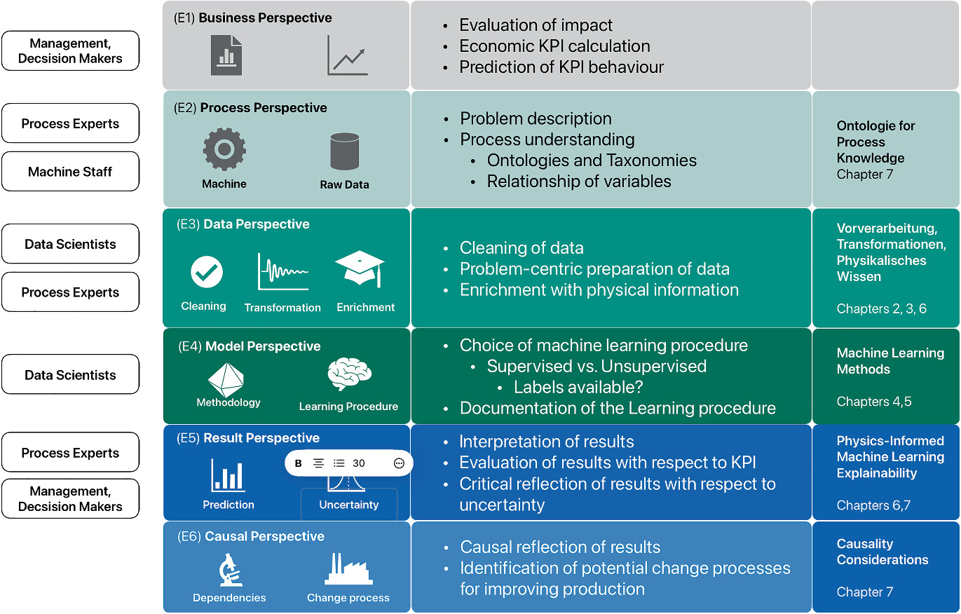
The six levels of explainability (E1–E6)

• A structured framework for matching explanation depth to audience and purpose.
• Each level addresses a different question about the model and its predictions.
• Comprehensive explainability requires addressing all six levels.
• Not every audience needs every level — match the explanation to the recipient (Neuer et al. 2024).

Overview of the six levels of explainability (E1–E6) (Neuer et al. 2024)

• This is the organizing skeleton of the unit’s core — have them photograph it. The next six slides are one level each; the “match level to audience” table later is this slide cashed out. Say “everything for the next 20 minutes hangs on these six hooks” so they file the detail correctly.
• The non-obvious structural point to state: E1→E6 is ordered from data to decision, i.e. it walks the same pipeline the whole course followed (data → model → prediction → action). It is not an arbitrary list; it is the lifecycle, made into an explanation checklist.
• The sentence that prevents the most confusion: you do not owe every audience every level — comprehensive explainability means the levels exist and are documented, not that every recipient reads all six. This kills the “this is impossibly much work” reaction and sets up the audience-matching table.
• Materials-cohort framing: position E1–E6 as the structure of a model card / qualification dossier for an industrial ML system — the document a regulator or auditor walks top to bottom. Make it a deliverable, not a taxonomy.
• Transition: “Bottom of the stack, where every model’s credibility actually starts — the data.” → E1.

E1: Data level

• Question: “What data was used?”
• Covers: data provenance, quality, completeness, representativeness, biases.
• Why it matters: a model is only as good as its data — garbage in, garbage out.
• Output: data documentation, distribution plots, missing data reports.

• Set the rhythm for the E1–E6 block: each slide is question → covers → why → output. Deliver them briskly and parallel; the pedagogical value is the pattern, so don’t let any single level sprawl. Spend the saved time on E5 and the audience table, which are where the exam questions live.
• E1 is the level engineers most underrate and regulators most scrutinize — say it plainly: a flawless model on biased data is a confident wrong answer with paperwork. “Garbage in, garbage out” is not folklore here; it is the first thing an EU AI Act audit asks for.
• Materials anchor that makes it bite: a fatigue model trained only on samples from one supplier’s heat-treatment furnace is representative of that furnace, not of the alloy. E1 is where you would have documented that and caught it before deployment. Tie forward: this is exactly the confounder we revisit in §9.
• Connect to Unit 12: E1 documents the support of the training distribution; data-manifold limits and OOD detection (§10 today) are the test-time enforcement of what E1 declared. E1 says “here is where I have data”; the manifold slides say “refuse to predict elsewhere.” Same boundary, declared then policed.
• Transition: “Data is necessary but not sufficient — what physical process does this model even claim to be about?” → E2.

E2: Process level

• Question: “What physical process does this model relate to?”
• Covers: the engineering context, the physical system, the measurement setup.
• Why it matters: predictions must be interpreted in the context of the physical process.
• Output: process flow diagrams, variable definitions, physical constraints.

• E2 is the level that distinguishes engineering ML from generic ML — say so. A Kaggle model needs E1/E3/E4; a deployed industrial model is meaningless without E2, because a prediction divorced from its physical process is just a number with no operating envelope.
• This is the slide where the ontology work pays off explicitly — the “process flow diagram + physical constraints” output is the process ontology from §4. Call that back: the earlier semantics block was not a detour; it was building the E2 artifact.
• Materials anchor: E2 is “this model predicts porosity for laser powder-bed fusion of Ti-6Al-4V at these scan parameters” — not “this model predicts porosity.” The qualifiers are the model’s domain of validity; omitting them is how models get used out of scope and fail in the field.
• Connect to Unit 13: E2’s “physical constraints” are exactly the conservation laws a PINN would enforce in the loss. E2 is where you write them down so they can be checked; §10’s deductive reasoning is where the model’s explanation is tested against them. Documentation now, enforcement later.
• Transition: “Process fixed — now the question engineers ask first: which inputs actually drive it?” → E3.

E3: Feature level

• Question: “Which input features matter most?”
• Covers: feature importance, feature selection rationale, sensitivity analysis.
• Why it matters: identifies which measurements drive predictions — guides data collection and process control.
• Output: feature importance rankings, sensitivity plots.

• Flag E3 as the highest-yield level in the unit: it is where the only examinable computation lives (the sensitivity formula in §8), and where SHAP/Integrated Gradients all land. Tell students “E3 is the level you will actually be tested on producing, not just describing.”
• The engineering payoff to land: feature importance is not a curiosity — it tells you which measurement to keep funding and which process knob to instrument. Low-importance, expensive-to-measure features are candidates to drop; high-importance ones justify better sensors. Explanation drives capital decisions.
• Plant the §8 caveat now so it doesn’t surprise them later: “we will spend real time on E3, and the punchline will be that feature importance reveals association, not mechanism — it answers ‘what did the model use,’ never ‘what causes the outcome.’” Setting this expectation early makes the causality section land instead of feeling like a reversal.
• Misconception to preempt: students conflate “the model relies on feature X” with “X matters physically.” E3 is strictly the former. The bridge to the latter is the ontology consistency check (§10) — name the link.
• Transition: “Inputs settled — now look at the box itself: how does the model work?” → E4.

E4: Model level

• Question: “How does the model work?”
• Covers: architecture description, hyperparameter choices, training protocol, convergence diagnostics.
• Why it matters: enables reproduction, debugging, and comparison with alternative models.
• Output: model documentation, training curves, architecture diagrams.

• Reframe E4 from “boring documentation” to reproducibility as a scientific obligation — this is the level that connects directly to the §2 falsifiability argument. An unreproducible model cannot be independently tested, so it cannot be falsified, so it is not science. E4 is where that promise is kept.
• The callback to make explicit: “what does it optimize” (loss, Unit 1), “how does it train” (optimizer/landscape, Unit 6), “did it converge” (training curves, Unit 6) — E4 is literally the documentation of everything from the optimization half of the course. Tell them E4 is where Units 1 and 6 become an audit artifact.
• Honest nuance for strong students: E4 explains the architecture and training procedure, which is not the same as explaining the learned function. A fully documented 50-layer net is reproducible but still a black box at E5. This is precisely the gap mechanistic interpretability (§8) tries to close — foreshadow it.
• Misconception to preempt: “E4 = interpretability.” No — documenting hyperparameters does not make the model transparent; it makes the process transparent. Keep the §2 vocabulary clean: E4 is reproducibility, not interpretability.
• Transition: “Process, features, model — but the engineer in the field cares about this one prediction. Why this output for this sample?” → E5.

E5: Prediction level

• Question: “Why this specific prediction?”
• Covers: local explanations for individual predictions.
• Methods: SHAP (Shapley values), Integrated Gradients, perturbation analysis.
• Output: “This sample is predicted high-strength because carbon content is high and grain size is small.”

• E5 is the conceptual center of the whole unit — emphasize the shift: E1–E4 explain the model globally and once; E5 explains one prediction, freshly, every time. This local/global distinction is the spine of the entire sensitivity + SHAP block that follows; say “the next eight slides are all techniques for doing E5.”
• The named methods are not a list to memorize in passing — they are forward pointers: perturbation (next slide), SHAP (waterfall/beeswarm slides), Integrated Gradients (its own slide). Tell them E5 is where today’s machinery gets built; everything from here to §8 is E5 made operational.
• The honest caveat to plant: every E5 method produces an explanation that is locally faithful to the model, not necessarily true about the world. “Carbon is high → high strength” might be the model’s logic on a confounded dataset. Connect to §9 — E5 explanations inherit every spurious correlation the model learned.
• Connect to Unit 12: a complete E5 statement is attribution + calibrated confidence — “high-strength because of carbon (SHAP), and I am 85% sure (UQ).” Reinforce the unit’s thesis: explanation without confidence, or confidence without explanation, is half a deliverable.
• Transition: “An attribution still isn’t an action. The operator doesn’t want ‘carbon mattered’ — they want ‘do this.’ That’s E6.” → E6.

E6: Decision level

• Question: “What action should be taken?”
• Covers: mapping predictions to actionable recommendations with confidence.
• Why it matters: the ultimate purpose of the model is to inform decisions.
• Output: “Increase sintering temperature by 20°C (confidence: 85%).”

• E6 is the level that justifies the entire course existing — say it directly: every unit, from loss minimization to UQ, exists so that a human can take a defensible action. A model that stops at E5 has produced understanding; only E6 produces value. End the E1–E6 ladder on that note.
• The structure of the E6 output is the lesson: it is imperative + magnitude + confidence. “Increase sintering temperature by 20 °C (85%).” Each piece traces back — the imperative needs causal validity (§9), the magnitude needs the model, the confidence is the Unit 12 callback. E6 is where explanation and uncertainty finally fuse into one sentence.
• The deep caveat to land hard: E6 makes a prescriptive, interventional claim (“change X and Y will change”). That requires causation, not the correlation E3/E5 give you. This is the single most important setup for the §9 causality block — say explicitly “an E6 recommendation built on a correlational model is the most dangerous artifact in this unit; we return to exactly this in 15 minutes.”
• Materials anchor: contrast a safe E6 (“adjust within the qualified process window, 90% confident”) with a reckless one (“extrapolate composition 30% beyond any training sample”). The confidence number is what makes E6 honest rather than authoritative-sounding.
• Transition: “Six levels exist — but no one needs all six. Who gets what?” → matching level to audience.

Matching level to audience

Audience	Primary levels	Example explanation
Operator	E2 + E6	“Adjust temperature; model is 90% confident”
Data scientist	E3 + E4	“Feature X has highest SHAP value; 3-layer MLP”
Regulator	E1 + E5	“Data from 500 samples; prediction driven by grain size”
Scientist	All	Full documentation and methodology

• Different stakeholders require different depth and focus.
• Explanations must be tailored to the user’s technical background and decision-making needs.

• This table is the payoff of the entire E1–E6 ladder and of the “who needs explanations” slide from §2 — point back to both. It converts an abstract framework into a deployable spec: for each stakeholder, exactly which levels to produce. This is the slide students should reproduce on the exam if asked “how do you scope an explainability deliverable.”
• Walk one row aloud as a story, not a lookup: the operator gets E2+E6 because they need context and an action, not SHAP values they cannot act on; the regulator gets E1+E5 because they audit data provenance and per-decision justification, not architecture. The lesson is that the correct explanation is recipient-relative — there is no universally best explanation.
• The misconception to kill: “give everyone everything to be safe.” That fails twice — it buries the operator’s action and still may not satisfy the regulator’s specific provenance demand. Precision of explanation is a design constraint, like latency; over-delivery is a failure mode, not caution.
• Engineering reframe: this table is a requirements document. Treat audience-level mapping as you would a sensor spec — agreed before the model is built, not improvised after. Tie to E2/E4: these get documented once; E5/E6 are generated per query.
• Transition: “The table promises E3/E5 explanations. Time to actually build one — the simplest faithful method: perturbation.” → perturbation-based sensitivity.

Perturbation-based sensitivity analysis

• Perturb one input feature by \(\); observe the change in output:

\[ S_j = \frac{|f(\mathbf{x} + \Delta \mathbf{e}_j) - f(\mathbf{x})|}{|\Delta|} \]

• High sensitivity: the output changes strongly when this feature is perturbed.
• Low sensitivity: the feature has little effect on the prediction.
• Simple, model-agnostic, and intuitive.

• This is the one formula in the unit students must be able to write from memory and interpret — slow down and put it on the chalkboard. Read it as a finite-difference derivative: \(S_j\) is just \(|f/x_j|\) estimated by a one-sided difference. Naming it “a numerical directional derivative of the model” makes it click for a cohort that has done calculus (Unit 3).
• Derive the intuition, don’t assert it: perturb only \(x_j\) (the \(_j\) one-hot step), hold all else fixed, measure output response per unit input. High \(S_j\) = steep slope along that axis = the model leans on that feature here. This is E3/E5 made concrete — point back: “this is the machinery the audience table promised.”
• “Model-agnostic” is the headline selling point — emphasize it: this works on a random forest, a 50-layer net, or a black-box vendor API, because it only needs forward evaluations, no gradients, no internals. That is exactly why it is the universal first-line explainability tool despite its flaws.
• Plant the three caveats now so §8’s “limitations” slide is a payoff, not a surprise: (1) it is local — one point, one direction; (2) it is one-at-a-time — blind to interactions; (3) it measures association, never mechanism. Write “remember these three” on the board.
• Likely exam question: “given \(f\), \(\), \(\), compute \(S_j\) for two features and rank them.” Tell them so. Transition: “One number at one point — but which question are you answering, global or local?” → global vs local.

Global vs local sensitivity

• Global sensitivity: average \(S_j\) across many data points — which features matter on average.
• Local sensitivity: \(S_j\) at a specific point — which features matter for this prediction.
• Global sensitivity guides feature selection; local sensitivity explains individual predictions.

• This is the same global/local axis that organizes the SHAP slides (beeswarm = global, waterfall = local) and earlier separated E3 from E5 — make the recurrence explicit so students see it is one idea, not three. “You will meet this distinction a third time in five minutes; it is the backbone of the whole E5 block.”
• The crisp operational rule to land: average over the dataset → which features matter for the model in general → drives feature selection and sensor budgeting (an E3, design-time decision). Evaluate at one point → why this part was flagged → drives the per-case justification a regulator or operator needs (an E5, run-time decision). Different audience, different computation, same formula.
• The misconception to kill: students assume the globally important feature explains every individual prediction. Counterexample to say aloud — grain size dominates on average, but for one specific high-carbon sample carbon content is the local driver and grain size is flat. Averaging hides exactly the case-specific story that an audit demands.
• Connect to Unit 8: global sensitivity is a feature-selection signal, so it ties to the bias–variance/regularization story — dropping low-global-sensitivity features is capacity control informed by the model, not a generic penalty. Name the link; it reinforces that explainability and generalization are coupled.
• Transition: “Theory done — now do it on a real model and see what the curves actually look like.” → sensitivity analysis in practice.

Sensitivity analysis in practice

• Vary each feature by \(%\) (or \(\)) while holding others constant.
• Record the output change for each perturbation.
• Rank features by average output sensitivity.
• Visualize as a bar chart: “tornado plot” showing feature sensitivities.

Perturbation scan of a decision tree: true function (black) vs. sensitivity scan (red crosses) (Neuer et al. 2024)

• Read the figure carefully — it is doing more than illustrating the recipe. The red scan tracks the black true function in steps, exposing that a decision tree is piecewise constant: sensitivity is ~0 inside a leaf and spikes at split boundaries. Use this to make the §8 limitations slide inevitable — “look, the local sensitivity here depends entirely on where you stand; that is the danger.”
• The “tornado plot” is the deliverable to name and sell: ±1σ (not a fixed ±10%) is the right perturbation because it makes features comparable across different units and scales — perturbing temperature by 10% and carbon by 10% is not a fair comparison; perturbing each by its own σ is. State the normalization reason explicitly; students miss it.
• Practical engineering point: this is a few-dozen forward passes per feature — cheap enough to run on any model in a notebook before lunch. Contrast with SHAP (next) which is exponentially more expensive. The recurring theme of the unit: pick the cheapest method that gives a defensible answer for the decision at hand.
• Misconception to preempt: “the scan recovers the true function.” It recovers the model’s function, and only along axis-aligned 1-D slices. The black curve agreeing with red is a property of this clean example, not a guarantee. Tie to §9: faithful-to-model ≠ true.
• Transition: “Turn these scans into a ranking — and then immediately stress-test what the ranking does and doesn’t mean.” → feature importance from sensitivity.

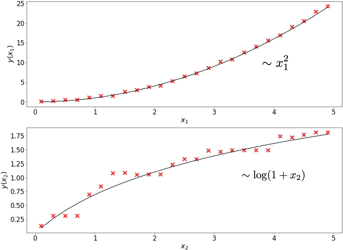
Feature importance from sensitivity

• High sensitivity \(\) important feature — changes in it strongly affect predictions.
• Low sensitivity \(\) unimportant feature — can potentially be removed.
• But: sensitivity alone does not imply causation — it reveals association.
• Combine with domain knowledge to interpret importance.

Main effects (partial-dependence-style) for a random forest model — flat curves indicate unimportant features (McClarren 2021)

• The third bullet is the moral of the entire E3/sensitivity block — say it slowly and write it: sensitivity reveals association, not causation. A feature can be highly sensitive because it is a genuine driver, or because it proxies a confounder the model latched onto. The scan cannot tell which. This is the explicit bridge into §9; announce it as such.
• Teach the figure as a reading skill: a flat main-effect curve = the model’s output is invariant to that feature = low importance = a drop candidate. A sloped or wiggly curve = the model uses it. This is partial-dependence intuition and connects back to Unit 8 feature selection — same decision, now explanation-driven.
• The dangerous engineering mistake to name explicitly: dropping a feature because sensitivity is low. Two traps — (1) it may be low only at this operating point (local!), high elsewhere; (2) it may be a true cause masked by a correlated proxy the model preferred. Removing it can silently break the model outside the tested region.
• Reinforce the unit thesis: importance must be read with domain knowledge (the ontology, §4/§10), not instead of it. A ranking that contradicts known physics is a finding about the data or model, not a discovery about the world. Pair every importance plot with the ontology consistency check.
• Transition: “We’ve hinted at the cracks three times. Now name them all at once.” → sensitivity analysis: limitations.

Sensitivity analysis: limitations

• Assumes independence: one-at-a-time perturbation misses feature interactions.
• Linear approximation: sensitivity at one point may not represent the full landscape.
• No causal information: sensitivity shows association, not mechanism.
• For interactions: use Sobol indices or SHAP (more expensive, more informative).

• This is the slide that earns the previous five — deliver it as the deliberate payoff of every caveat you planted, not as a downer. Each limitation maps to a real failure: “assumes independence” → misses synergistic alloying effects; “linear approximation” → wrong wherever the model is nonlinear (i.e. everywhere interesting); “no causal info” → the §9 trap. Name the materials consequence for each, don’t leave them abstract.
• Hammer the interactions point with a physical example: hardness depends on carbon and tempering temperature jointly — perturbing each alone can show both as mildly important while their interaction dominates. One-at-a-time sensitivity is structurally blind to this. This is why Sobol/SHAP exist; the next slide is the answer to this exact gap.
• Calibrate honestly: this does not make perturbation worthless — it makes it a screening tool. The engineering pattern is cheap screen first (perturbation), then expensive principled attribution (SHAP) only where stakes justify the cost. Reuse the unit’s recurring “cheapest defensible method” line.
• Connect “linear approximation” back to the §8 figure: the decision-tree scan was piecewise constant, so the local slope was meaningless inside leaves and undefined at splits — a concrete instance of the limitation, not just a caveat. Point at the prior slide.
• Transition: “Sobol is one fix; the one you’ll actually use in 2026 is SHAP — game theory applied to attribution.” → beyond perturbation: SHAP.

Beyond perturbation: SHAP values (brief)

• SHAP (SHapley Additive exPlanations): allocates prediction contribution to each feature using game theory.
• Based on Shapley values: fair allocation of the “payout” (prediction) to “players” (features).
• Accounts for feature interactions.
• Computationally expensive but provides the most principled feature attribution.

• Keep the game-theory framing one level deep but make it stick: features are “players,” the prediction minus the baseline is the “payout,” and a feature’s SHAP value is its average marginal contribution over all orders in which features could be added. That averaging-over-coalitions is exactly what fixes the one-at-a-time blindness from the limitations slide — say “this is the principled answer to the interaction problem we just named.”
• State the uniqueness result as the reason SHAP won: Shapley values are the only attribution satisfying efficiency, symmetry, dummy, and additivity. “Most principled” is not marketing — it is a theorem. This is the exam-quotable sentence; flag it.
• Be honest about the cost so the unit’s cost/benefit theme stays consistent: exact Shapley is exponential in #features; in practice you use approximations (KernelSHAP, TreeSHAP). TreeSHAP is exact and fast for tree ensembles — tie back to Unit 8, since their tabular materials models are usually gradient-boosted trees, so SHAP is genuinely cheap for them. This makes it the realistic default, not a luxury.
• The caveat that survives even SHAP: it is faithful to the model, so it still explains a confounded model’s confounded logic perfectly. Principled attribution does not buy causation. Reinforce — this is why §9 exists and why SHAP plots must be read against the ontology.
• Transition: “Two plots you must be able to read on sight — start with the single-prediction one (E5).” → SHAP waterfall.

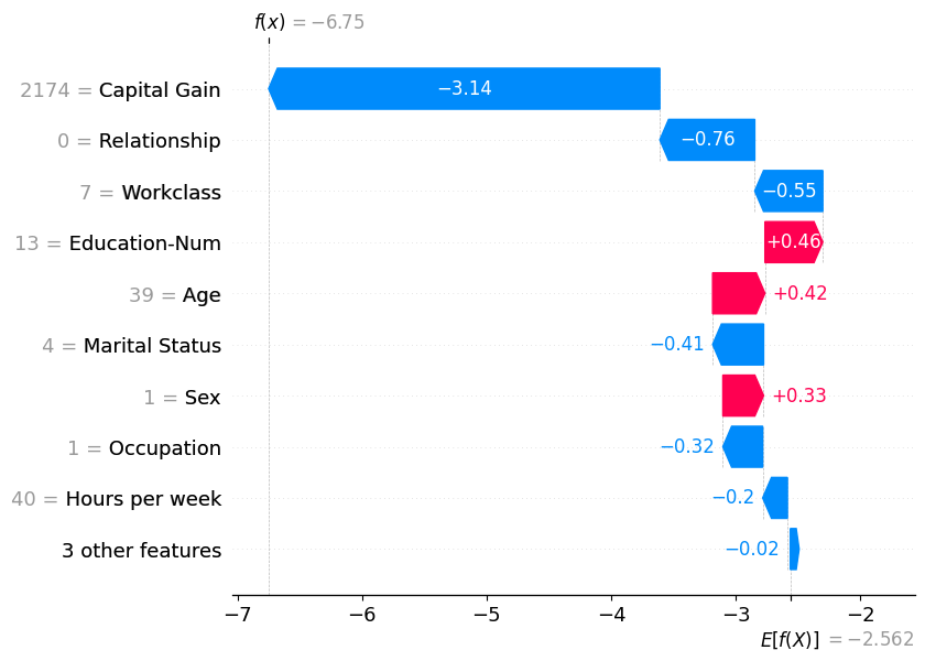
SHAP waterfall plot — explaining one prediction

• A waterfall plot decomposes a single prediction into per-feature contributions.
• Starting from the expected model output \(\mathbb{E}[f(x)]\), each bar adds or subtracts the SHAP value of one feature.
• Red bars push the prediction higher; blue bars push it lower.
• The final value at the top is the model output for that instance (Lundberg and Lee 2017).

SHAP waterfall plot: each feature’s contribution to a single prediction, from the SHAP Python library (MIT license)

• Teach this as a reading exercise, not a concept — students will see this exact plot in their own notebooks and in papers. Walk it bottom-to-top live: start at the base value \([f(x)]\) (“what the model predicts knowing nothing about this sample”), then each bar is one feature moving the prediction, ending at the actual output \(f(x)\) at the top. The visual is the additivity axiom from the previous slide — point that out.
• The single most important sentence: this is the canonical E5 artifact and the literal answer to “why this prediction?” The waterfall is what you hand a regulator or a domain expert to justify one decision. Connect explicitly to the audience table — “this is the E5 in the regulator’s E1+E5 row.”
• Make red/blue unambiguous and physical: red pushes the prediction up, blue down; bar length = magnitude of that feature’s contribution for this sample. Re-anchor in materials: “this billet is predicted high-strength: +carbon, +cooling-rate (red); −grain-size pushed back (blue).” Numbers, not adjectives.
• The caveat to keep visible: the waterfall is exact and self-consistent with respect to the model — it sums perfectly to \(f(x)\). It says nothing about whether the model’s reasoning is physically causal. A confounded model produces an equally tidy, equally wrong waterfall. Tie to §9 again.
• Transition: “One sample is E5. Aggregate thousands and you get a global, E3 view — the beeswarm.” → SHAP beeswarm.

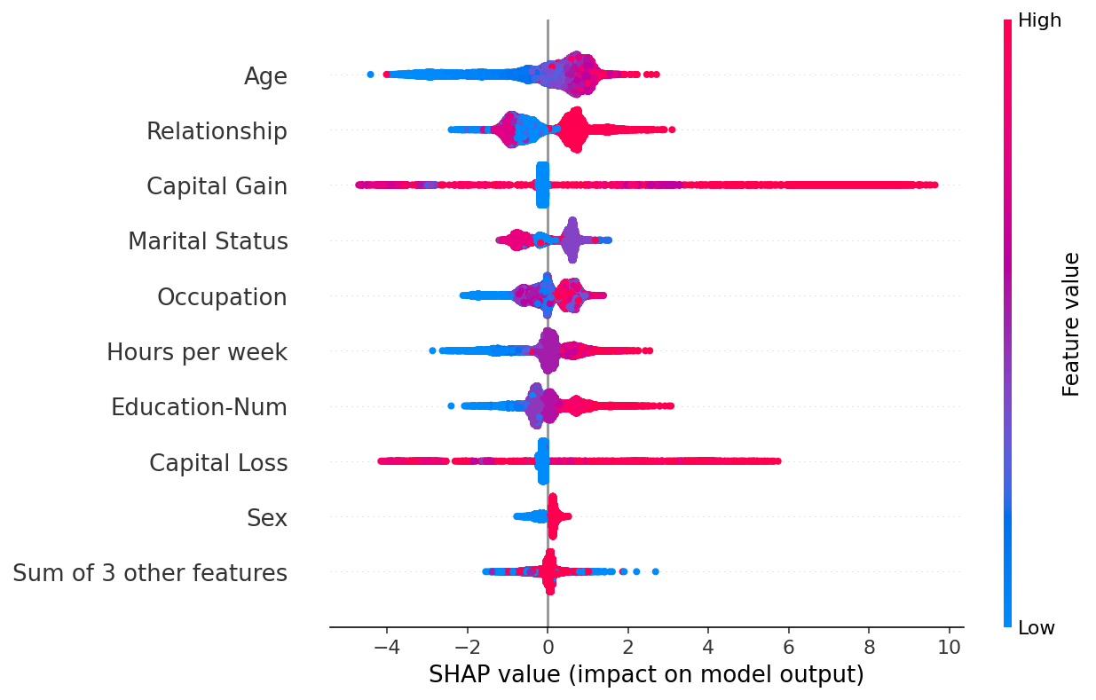
SHAP beeswarm plot — global feature importance

• A beeswarm plot summarises SHAP values across the entire dataset.
• Each dot is one data point; the x-axis shows the SHAP value (impact on prediction).
• Colour encodes the feature value (red = high, blue = low).
• Features are ranked by mean |SHAP|, giving a global importance ranking with local detail (Lundberg and Lee 2017).

SHAP beeswarm (summary) plot: global feature importance with individual-point detail, from the SHAP Python library (MIT license)

• Read it as a two-channel plot — this is the skill students must leave with. Vertical: features ranked by mean |SHAP| → the global E3 importance ranking. Horizontal spread of dots: per-sample SHAP → the local E5 detail. Colour: the feature’s value (red high, blue low). One plot, global + local at once — say “this is why beeswarm is the single most information-dense explainability figure you will produce.”
• Teach them to read direction of effect from colour, which the bare ranking hides: if a feature’s high values (red) sit on the positive-SHAP side, “more of it → higher prediction” — and you can check that sign against the ontology/physics. A red-on-negative pattern that contradicts known physics is a §10 falsification flag, surfaced visually.
• Contrast with the previous slide to lock the global/local axis one final time: waterfall = one sample, E5, hand to a regulator; beeswarm = whole dataset, E3, hand to a data scientist for feature selection. Same Shapley values, aggregated differently — point back to the audience table.
• The misconception to kill: a tall bar in the ranking means “globally important,” not “important for every sample.” The horizontal spread is precisely the evidence that one feature can dominate some predictions and be irrelevant to others — the exact point from the global-vs-local slide, now visible. Make them find a high-spread feature on the figure.
• Transition: “SHAP suits tabular materials data. For images and deep nets there’s a gradient-based cousin with its own axioms — Integrated Gradients.” → Integrated Gradients.

Integrated Gradients: attributing deep network predictions

• Integrated Gradients (Sundararajan et al. 2017): attributes a prediction to each input pixel by integrating gradients along a straight path from a baseline (black image) to the input.
• Satisfies two key axioms: Sensitivity (if input and baseline differ only in one feature, it receives non-zero attribution) and Implementation Invariance (functionally identical networks get the same attribution) (Sundararajan et al. 2017).
• Visualised as pixel-level heatmaps: positive attributions highlight features supporting the predicted class.

Integrated Gradients attribution heatmaps on ImageNet: positive attributions (gray scale) track discriminative object regions better than simple gradients (Sundararajan et al. 2017)

• Motivate IG by the failure it fixes: the naive idea is “just use the gradient \(f/x\) at the input as the attribution.” Say why that breaks — saturation. A confidently-classified image sits on a flat part of the function, so the local gradient is ~0 and a clearly-important pixel gets zero credit. IG’s fix: integrate the gradient along the straight path from a neutral baseline (black image) to the input. The path integral accumulates the credit the saturated endpoint hides.
• Keep it conceptual but precise — the cohort has done line integrals (Unit 3): IG is exactly the fundamental-theorem-of-calculus statement that the integrated gradient along a path equals the total change in \(f\). That single sentence makes the method feel inevitable rather than ad hoc; it also guarantees the completeness/efficiency property (attributions sum to \(f() - f()\)) — the same additivity idea as SHAP, now for deep nets.
• The two axioms are the exam-quotable content: Sensitivity (differ in one feature → nonzero attribution; this is precisely what bare gradients violate via saturation) and Implementation Invariance (two networks computing the same function get identical attributions — so the explanation depends on the function, not incidental architecture). Tell them these axioms are why IG is trusted, mirroring the Shapley uniqueness story.
• Make the baseline choice an explicit caveat, not a footnote: the attribution is relative to a baseline, and a bad baseline gives misleading maps. “Black image” works for natural images; for a micrograph or spectrum the right baseline is a domain question, not a default. This is the IG analogue of SHAP’s “explains the model, not the world.”
• Materials bridge to the next slide: SHAP/IG are input-side (“which inputs mattered”). Mechanistic interpretability asks the orthogonal question — “what is the network computing internally.” Set that pivot up; the next slide already carries its own detailed notes.

Mechanistic interpretability: reverse-engineering what a network actually learned

From attribution to internals

• SHAP and Integrated Gradients tell you which input features mattered for one prediction — an input-side view.
• Mechanistic interpretability asks a different question: what computation does this layer perform, and in what basis? It looks inside the network.
• For transformers, the residual stream is the natural object of study: every layer reads from it and writes to it. Treat it as the “thought-process bus” of the model.

Two ideas you should know

• Superposition (Elhage et al. 2022): networks store more features than they have neurons by overlapping them in directions that are not axis-aligned. Single neurons are usually polysemantic — they fire for many unrelated concepts.
• Sparse autoencoders (SAEs) (Bricken et al. 2023; Templeton et al. 2024): train a sparse-coding autoencoder on layer activations to recover an over-complete basis of monosemantic directions. Each SAE feature is an interpretable concept (e.g. “Golden Gate Bridge”, “buggy Python code”). Anthropic’s Scaling Monosemanticity (2024) extracted millions of such features from production Claude models.

• Status in 2026: SAE-based feature extraction is the dominant interpretability research direction for foundation models. Still emerging for vision/materials; a forward-looking topic, not yet a production tool.

• Why this slide sits here: SHAP and Integrated Gradients remain the applied tools you actually use on your own models today (they have largely displaced LIME as 2026 defaults). SAEs are the research-frontier tool for foundation-model interpretability. Students should leave knowing the latter exists and where it sits relative to the former.
• Pedagogical link to Unit 5: a sparse autoencoder is exactly the architecture from §D of Unit 5 (encoder + bottleneck + decoder) but with a sparsity penalty on the latent. The novelty here is what you train it on (activation vectors from a frozen LLM layer) and why (to discover the model’s internal feature basis).
• Why monosemanticity matters: a feature that fires for one concept (e.g. “Python code with off-by-one bugs”) can be intervened on — increase that feature’s activation in the residual stream and the model behaves accordingly. This unlocks targeted safety interventions and model debugging.
• Honest limits: SAE features are not unique (different sparsity hyperparameters give different bases), and not all features are interpretable. The method is young (2023+); coverage of model behaviour is still partial.
• Materials angle: when foundation models trained on micrographs become standard (Unit 9 territory), the same SAE techniques will apply for understanding what visual concepts they encode. Practical applications are emerging in 2025–2026.
• Genealogy: linear probes (Alain & Bengio 2017) and the broader circuits research program (Olah et al. 2020, transformer circuits) are the roots. Activation patching and attribution patching are the diagnostic verification tools that test whether an SAE feature is actually causally involved in a behaviour.

Causality vs correlation

• ML models find correlations: features that co-occur with the output.
• But correlation \(\) causation: confounders can create spurious patterns.
• Example: ice cream sales correlate with drowning rates (confounder: temperature).
• Causal claims require interventional data or domain knowledge.

• This is the conceptual climax of the whole explainability machinery — deliver it as the reckoning, not a new topic. Everything from E3 to SHAP to IG answers “what did the model use.” This slide says: that question, answered perfectly, still does not tell you “what causes the outcome.” Say it as a hard wall: no attribution method, however principled, crosses from correlation to causation.
• Run the ice-cream/drowning example as a live cold call before revealing the confounder — let them propose “ban ice cream,” then surface temperature as the common cause. The laugh is the point: it makes the materials version land harder, because that one is not funny.
• The materials version to deliver immediately after: a model finds furnace-ID strongly predicts part failure. The naive E6 action — “avoid furnace 3” — is wrong if furnace 3 merely processed the one bad powder lot. Same logical error as ice cream, but here it costs a production line. This is the §1 black-box anecdote paid off.
• The exam-grade sentence: causation needs an intervention (do(X), a designed experiment — a DOE) or domain knowledge (the ontology, the physics, Unit 13). Data alone, no matter how much, cannot distinguish a cause from a confounded proxy. Connect: this is why the ontology consistency check (§10) is not optional decoration — it is the only causal anchor a purely observational model has.
• Transition: “In manufacturing we do know the causal direction — physics gives it to us. That’s the process chain.” → causal process chains.

Causal process chains

• In manufacturing: Composition \(\to\) Processing \(\to\) Microstructure \(\to\) Properties.
• The arrow direction encodes causation: changing composition causes different microstructure.
• ML can model these links, but the causal direction is known from physics, not learned from data (Neuer et al. 2024).

Causal flow in an abstract process chain: detection algorithms (A3, A4) observe anomalies after they occur; prediction algorithms (A1, A2) anticipate them earlier (Neuer et al. 2024)

• This is the third return of the composition→processing→microstructure→properties chain (it appeared in §4 and §5) — name the recurrence and tell them why it keeps coming back: it is the one place where causal direction is known a priori from physics, not inferred from data. That makes it the safe ground from which to judge everything else.
• The key insight, and an exam favourite: ML can model any arrow, but the direction of the arrow is supplied by physics, never learned from observational data. The model fits \(P()\) equally well whether you believe composition causes properties or vice versa — only the ontology breaks the symmetry. This is the §9 thesis made concrete on their canonical example.
• Read the figure as the operational payoff: detection algorithms (A3/A4) sit downstream and react after the anomaly is already in the part; prediction algorithms (A1/A2) sit upstream and act before. Earlier in the causal chain = more expensive to instrument but more valuable, because you can still intervene. This sets up the very next slide’s detection-vs-prediction distinction.
• Tie back to the §5 ill-posedness slide: the arrows run forward for a reason — going against them (properties → composition) is the one-to-many inverse problem. The causal chain and the well-posedness argument are the same fact viewed twice.
• Transition: “That up/downstream split has a name and a sharp consequence for what ML can honestly claim.” → detection vs prediction.

Detection vs prediction

• Detection: “This sample has low hardness” — pattern recognition from measurements. ML excels here.
• Prediction: “Changing carbon content will increase hardness” — causal claim. Requires causal model.
• Most ML models perform detection (interpolation). Prediction (extrapolation with causal claims) requires more.

• Sharpen the vocabulary war here — this slide redefines two words students think they know. “Detection” = recognising a pattern within the training distribution (interpolation, correlational, ML’s home turf). “Prediction” in the causal sense = “if I change X, Y will change” (interventional, extrapolative). They will instinctively call any model output a “prediction”; force the distinction with the chalkboard.
• The sentence that ties the unit together: a SHAP/IG explanation justifies a detection perfectly and tells you nothing about whether the interventional claim holds. So a beautiful waterfall plot supporting “increase carbon to raise hardness” is still an unjustified causal leap if the model only ever did detection. This is the §8 machinery and the §9 warning colliding — make the collision explicit.
• Materials anchor with the cost attached: “this sample has low hardness” (detection — trust it, the model has seen this region) vs “raising carbon 0.1% will raise hardness here” (causal prediction — needs a DOE or the metallurgical phase diagram, i.e. domain knowledge). The first is a measurement surrogate; the second is an engineering decision with liability.
• Connect to Unit 12 and Unit 8: detection is reliable only inside the data manifold; the moment a “prediction” requires extrapolation, epistemic uncertainty must spike and the model must say “I don’t know.” Detection-vs-prediction is the causal face of the in-distribution-vs-extrapolation story; the next slide and the §10 manifold slides are its enforcement.
• Transition: “So where, concretely, does ML earn its keep in a causal chain — and where must it hand off?” → where ML adds value.

Where ML adds value in causal chains

• Within the training distribution: ML provides fast, accurate detection and interpolation.
• At the boundaries: uncertainty quantification (Unit 12) flags unreliable predictions.
• Beyond the distribution: causal models (physics, experiments) are needed.
• ML is most valuable when combined with domain knowledge, not as a replacement for it.

• This slide is the constructive resolution after two slides of warnings — deliver it with that arc: “we’ve said what ML can’t do; here is precisely where it is the right tool.” Students should leave with a decision rule, not pessimism.
• Read the three regimes as a single map keyed to Unit 12’s uncertainty picture: inside the manifold → ML is fast, accurate, and the best tool — use it without apology. At the boundary → ML’s job is to raise its hand via UQ (the explicit Unit 12 callback — epistemic uncertainty must balloon here). Beyond → hand off to physics/experiment (Unit 13). The decision boundary literally is the uncertainty estimate.
• The final bullet is the thesis of the back half of the entire course — say it as such: ML + domain knowledge > ML alone, and > domain knowledge alone. Position this as the answer to the §1 question “can we trust our models?”: yes, conditionally, inside this map, with this handoff discipline.
• Misconception to preempt: the strong-student instinct that “with enough data ML replaces the physics.” Counter directly — more data extends the manifold but never converts correlation to causation or makes extrapolation safe. The handoff is structural, not a temporary limitation of dataset size.
• Transition: “We keep invoking ‘domain knowledge’ as the causal anchor. Time to operationalise it — the ontology as an automatic falsification check.” → deductive reasoning with ontologies.

Deductive reasoning with ontologies

• If the ontology states “grain size affects yield strength” but the model assigns zero importance to grain size:
  • Either the data lacks variation in grain size, or
  • The model has a problem.
• Ontological consistency checking catches such issues automatically.
• This connects explainability to domain validation.

• This is the slide that closes the loop opened in §2 — say so explicitly: “remember the falsifiability promise from the start of the lecture? This is the machine that keeps it.” The ontology turns an abstract Popperian principle into an automated unit test on the model’s explanation.
• Walk the example as a logical syllogism on the board: ontology asserts “grain size affects yield strength”; the model’s SHAP/sensitivity assigns grain size ≈ 0 importance; therefore something is wrong. Then teach the diagnostic fork — it is exactly two cases: (1) the data lacks variation in grain size (so the model couldn’t learn the effect — an E1 failure), or (2) the model is broken/confounded. Naming both branches is the examinable skill.
• The deep point: this is deduction layered on top of induction. The model induces patterns from data; the ontology deduces what must hold from physics; the contradiction between them is information neither could produce alone. This is the concrete mechanism behind “ML + domain knowledge > either alone” from the previous slide.
• Honest limit to state: the check is sound but incomplete — a contradiction always means a real problem, but the absence of contradictions does not certify the model (the ontology only covers the relations you bothered to encode). Frame it as a safety net that catches known failure modes, not a correctness proof.
• Transition: “Let’s make sure the causality block actually landed —” → checkpoint.

Checkpoint: causality

• Question: Your model finds that ice cream sales predict drowning rates. What’s the issue?

• Answer: Confounding variable — temperature causes both. The model found a correlation, not a causal relationship.

• Cold call before revealing — and don’t accept “correlation isn’t causation” as a full answer. Push for the mechanism word: confounder, and the requirement that they name it (temperature) and draw the fork (temperature → ice cream; temperature → drowning; no arrow between the two). Naming + diagramming the confounder is the gradeable skill, not reciting the slogan.
• Immediately demand the materials transfer — that is the real test: ask the room for an analogous confounder in a process dataset (ambient humidity driving both a sensor reading and a defect rate; a shared upstream lot; a campaign/seasonal effect). If they can produce one unprompted, the §9 block succeeded; if not, supply one and slow down.
• This is the highest-probability conceptual exam question in the unit — tell them so plainly. “Identify the confounder and explain why feature importance is misleading here” is the canonical format; the answer template is confounder name → fork structure → why the model’s attribution is faithful-but-wrong.
• Recovery valve: this checkpoint and the semantics one are your two compressible slides. If on time, use it to resurface the §1 furnace-ID anecdote and the §10 ontology check (“how would the consistency check have caught this?”) — that closes three threads at once.
• Transition: “Confounding is one way trust breaks. The other is geometric — leaving the data manifold.” → data manifold limits.

Data manifold limits

• ML models are only reliable within the data manifold (training distribution).
• Extrapolation: predicting outside the training range is unreliable — the model has no information there.
• Detection: use latent space density (Unit 9), reconstruction error (Unit 5), GP uncertainty (Unit 12).
• Never trust predictions in regions where the model has not seen data.

• This slide is a deliberate convergence point — three earlier units land here at once. Make the callbacks explicit on the board: latent-space density (Unit 9), reconstruction error (Unit 5 autoencoders), GP uncertainty (Unit 12). Same idea, three detectors: “am I still standing on the training manifold?” Students should see these were not separate tricks but one principle.
• The geometric intuition to draw: training data lives on a thin manifold inside a high-dimensional input space; the model is only constrained on that manifold. Off it, the function is whatever the architecture’s inductive bias happens to extrapolate — confident, smooth, and unmoored from any evidence. “The model is most dangerous exactly where it is most confident-sounding.”
• The last bullet is the single most important operational rule of the whole trust block — say it as a hard discipline, not advice: a prediction outside the training manifold is not a worse prediction, it is not a prediction at all. The correct output there is an abstention, not a number.
• Materials anchor: a fatigue model trained at 20–200 MPa asked about 400 MPa will return a clean number with no warning unless you instrument the manifold check. The high-strength regime they actually care about is usually the extrapolative one — this is not an edge case, it is the typical case in materials discovery.
• Transition: “If we are on the manifold, explanations can become actionable — counterfactuals tell the user what to change.” → counterfactual explanations.

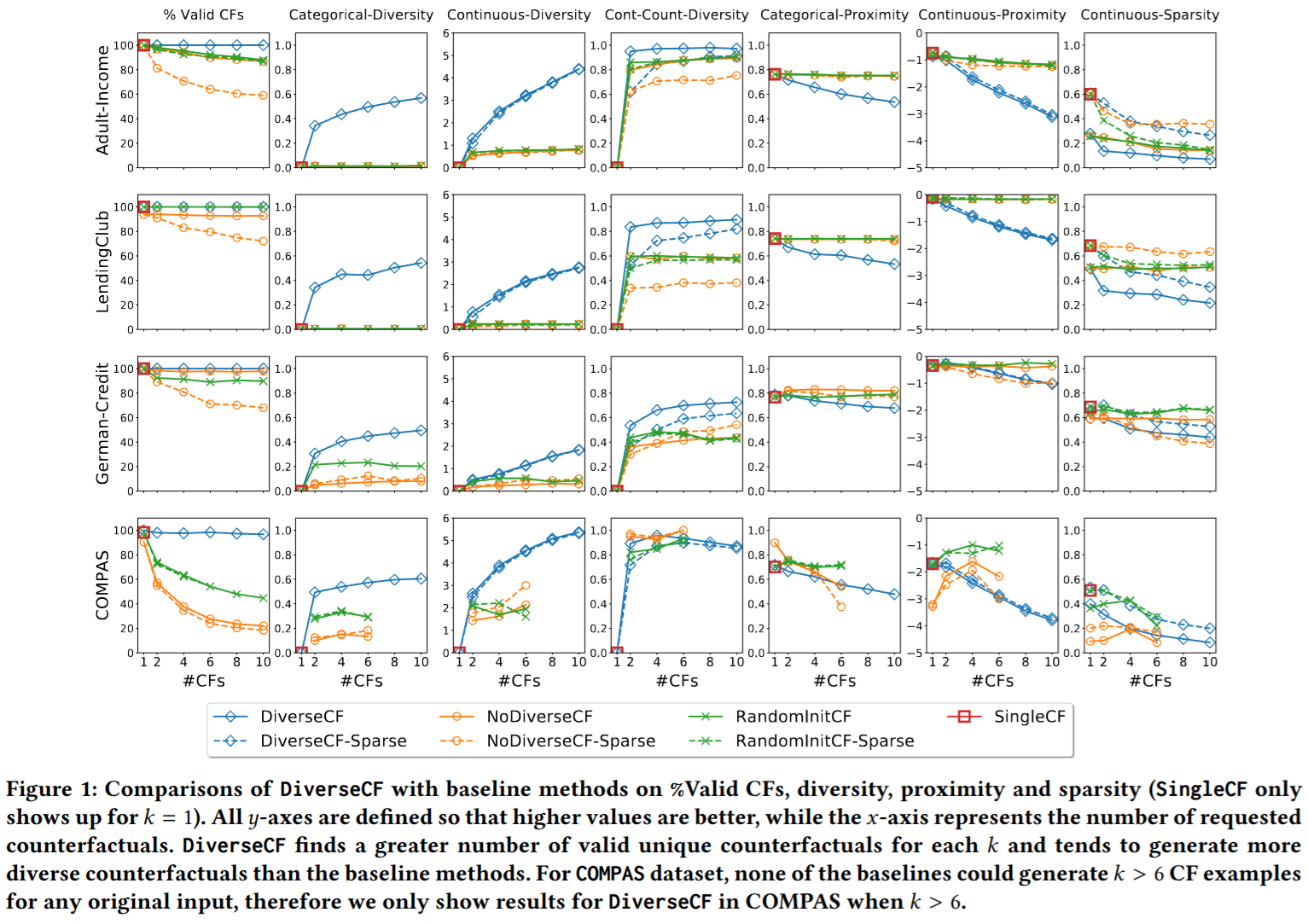
Counterfactual explanations: “what if?”

• A counterfactual explanation answers: “what is the smallest change to the input that would flip the prediction?”
• Example: “Your loan was denied. If your income were €5 000 higher and your debt €2 000 lower, it would be approved.”
• Counterfactuals are actionable: they tell users what to change, not just what mattered.
• DiCE (Mothilal et al. 2020) generates diverse counterfactuals so users see a range of valid alternatives (Mothilal et al. 2020).

DiCE: diversity and proximity metrics for generated counterfactual explanations across datasets and baseline methods (Mothilal et al. 2020)

• Frame counterfactuals as the mirror image of SHAP — this contrast is the slide’s main idea. SHAP/IG answer “why this outcome?” (attribution, backward-looking). A counterfactual answers “what is the smallest change that flips it?” (recourse, forward-looking, actionable). Recourse is what an operator actually needs — connect straight back to the E6/audience table: this is the E6 explanation, finally constructive.
• The loan example is the clearest, but immediately translate to materials so it isn’t an HR anecdote: “this billet is predicted to fail QC; the nearest passing configuration is cooling-rate +15 °C/s and grain-size −5 µm.” That is a process setpoint, not just an explanation — the whole point of the unit’s E6 level.
• The two competing objectives are the examinable concept and the reason DiCE exists: a counterfactual must be proximal (a small, cheap change) and the set must be diverse (several genuinely different routes, not ten near-duplicates). Read the figure as exactly this trade-off across methods; DiCE’s contribution is jointly optimising both.
• The honest caveat that ties to §9 — say it explicitly: a counterfactual is only an actionable recommendation if the changed feature is genuinely causal and manipulable. “Lower the grain size” is actionable; “be a different alloy” is not. A counterfactual on a confounded feature is the §9 trap wearing a constructive mask. Counterfactual recourse inherits every causality caveat from the last block.
• Transition: “Actionability raises a sharper question — actionable and fair for whom? Bias is a trust failure too.” → fairness and bias.

Fairness and bias in ML predictions

• ML models can perpetuate or amplify societal biases present in training data.
• Equalized odds (Hardt et al. 2016): a predictor is fair if it has equal true-positive and false-positive rates across protected groups (e.g. race, gender).
• Equal opportunity: the weaker condition of equal true-positive rates only.
• Figure 1 shows the ROC polytope of achievable (FPR, TPR) pairs per group — fairness requires operating at the same point on both group-specific ROC curves (Hardt et al. 2016).

Hardt et al. 2016 Fig 1: achievable (FPR, TPR) regions for two demographic groups; equalized odds requires the same operating point for both (Hardt et al. 2016)

• Anticipate the “this is a materials course, why fairness?” reaction and answer it head-on: fairness is the same mathematical object as the §9 confounder, just with a protected attribute as the variable. A model that keys on a proxy for supplier, region, or operator is bias in exactly the technical sense — the regulatory framing (EU AI Act) makes it non-optional regardless of domain. This is a trust failure, not a social-studies digression.
• Define the metrics precisely because students blur them: equalized odds = equal TPR and equal FPR across groups; equal opportunity = the weaker condition, equal TPR only. The relationship is the exam point — equal opportunity is equalized odds with the FPR constraint dropped. Make them state which is stronger and why you might settle for the weaker one.
• Teach the figure as a geometry argument, which is the real content: each group has its own ROC curve, so its own achievable (FPR, TPR) polytope. Fairness = picking an operating point that lies in both regions simultaneously. The visual punchline: this is generally not the accuracy-optimal point for either group — fairness has a quantified cost, it is a constrained optimisation, not a free add-on.
• The impossibility result to mention (don’t derive): you cannot in general satisfy all reasonable fairness criteria at once (calibration vs equalized odds conflict unless base rates are equal). The honest lesson, consistent with the unit: fairness is a choice of which criterion, made explicit and defended — exactly like choosing a loss function in Unit 1.
• Transition: “Bias, confounding, extrapolation — all trust failures. Two slides to make extrapolation operational: how do you actually detect it at runtime?” → detecting extrapolation.

Detecting extrapolation

• Latent space density (Unit 9): low density = far from training data = potential extrapolation.
• Reconstruction error (Unit 5 autoencoders): high error = input differs from learned patterns.
• GP uncertainty (Unit 12): wide uncertainty bands = no nearby training data.
• Ensemble disagreement: models disagree = uncertain = possible extrapolation.

• This is the operational cash-out of the “data manifold limits” slide — present it as a toolbox, four detectors for one question (“am I off the manifold?”), each from a different earlier unit. Make the callbacks loud: latent density (Unit 9), reconstruction error (Unit 5), GP variance (Unit 12), ensemble disagreement (Unit 8/12). The pedagogical message: the trust machinery was distributed across the course; this slide assembles it.
• Give the practical engineering guidance, not just the list: which detector you can afford depends on the model you already have. Trees → no natural reconstruction; use an ensemble (cheap, you may already have one). Autoencoder in the pipeline → reconstruction error is free. GP regression → variance is built in. The right detector is the one your existing model gives you for nearly zero extra cost — reuse the unit’s recurring “cheapest defensible method” line.
• The conceptual unifier to state: all four are proxies for low training-data density at the query point. They disagree precisely in the interesting cases, so in practice you threshold one and validate it on known-OOD examples — they are heuristics, not guarantees. Honesty about their failure modes is itself part of trustworthy ML.
• Misconception to preempt: “high model confidence means in-distribution.” The next slide’s whole point is that softmax confidence is not a reliable manifold detector — flag that this list deliberately does not include “trust the softmax,” and the next slide explains why that tempting shortcut fails.
• Transition: “The cheapest possible detector is the softmax you already have — does it work? Hendrycks & Gimpel give the honest baseline.” → OOD baseline.

Out-of-distribution detection: baseline approach

• Hendrycks & Gimpel (2017): the maximum softmax probability is a surprisingly effective OOD score.
• In-distribution examples typically produce high maximum softmax probabilities; OOD examples produce lower values.
• The method requires no modification to the trained network — only the softmax output at test time.
• AUROC (area under the ROC curve) measures detection quality: random = 50%, perfect = 100%.
• Limitation: softmax probabilities can be overconfident for OOD inputs far from the training manifold (Hendrycks and Gimpel 2017).

• Frame this as the baseline you must beat, and the cautionary tale — both at once. Hendrycks & Gimpel’s contribution is partly negative-result honesty: the dead-simple max-softmax-probability score is surprisingly decent, which is exactly why people lazily trust it — and why its failure mode is dangerous. Teach it as “the method everyone reaches for, and precisely where it betrays you.”
• Make AUROC concrete since it recurs from earlier units: it is the probability that a random in-distribution example gets a higher detection score than a random OOD example. 50% = coin flip, 100% = perfect separation. Tie back to the ROC geometry from the fairness slide two slides ago — same curve, different use.
• The limitation bullet is the real lesson and connects straight to Unit 12: a ReLU network’s softmax can be arbitrarily confident on inputs far from any training data — confidence is not calibrated off-manifold. This is the formal version of “the model is most dangerous where it is most confident-sounding” from the manifold slide. Calibrated UQ (Unit 12) exists precisely because this baseline is not enough.
• Engineering takeaway to state plainly: use max-softmax as a free first-pass screen, but never as the sole gate for a safety-relevant decision — pair it with a manifold/density detector from the previous slide. The honest combination, not the single cheap trick, is what trustworthy deployment looks like.
• Transition: “These failure modes all trace to one root — the model’s built-in assumptions. That is inductive bias, and it is the final lens on trust.” → inductive bias and trust.

Inductive bias and trust

• Every model has inductive bias — assumptions built into the model structure.
• Linear model: assumes linear relationships. NN: assumes smooth functions (spectral bias).
• Trust requires understanding what the model assumes and testing where those assumptions fail.
• Physics-informed models (Unit 13) make their assumptions explicit — a trust advantage.

• This is the unifying abstraction of the entire trust block — deliver it as “everything we just saw was one phenomenon.” Every model commits to assumptions before seeing data; that commitment is what lets it generalize and exactly what makes it fail off-distribution. No-free-lunch (Unit 8) restated: no inductive bias, no learning — and every bias is a place trust can break.
• Make the two examples precise and physical: a linear model’s bias is “the world is affine in these features” — it fails the moment the physics is nonlinear. A neural net’s bias is spectral bias (callback to Unit 4/6) — it prefers low-frequency, smooth functions, so it silently smooths over sharp transitions like a phase boundary. The danger is that both fail quietly, returning confident wrong answers, not errors.
• The payoff line and the bridge to Unit 13: trust is not “the model has no assumptions” (impossible) but “the assumptions are explicit and testable.” A PINN’s bias is written in the loss as a PDE you can read; a black-box net’s bias is implicit in weights you cannot. Explicit-and-wrong beats implicit-and-wrong because you can check the former — this is the same falsifiability theme from §2, now about the model’s priors rather than its predictions.
• Synthesis to state aloud: confounding (§9), off-manifold failure (§10), and miscalibrated confidence (Unit 12) are all inductive bias meeting a region where it is invalid. One root cause, three symptoms. This reframing is high-value for the exam’s “design/judgement” question.
• Transition: “If every model has a bias that can fail, the practical question is: enumerate exactly when you must not trust it.” → when models should NOT be trusted.

When models should NOT be trusted

• Extrapolation beyond the training distribution.
• Confounded features where correlation \(\) causation.
• Insufficient training data (high epistemic uncertainty).
• Missing physics (model violates known constraints).
• Poor calibration (predicted confidence does not match observed accuracy).

• Tell students to photograph this slide and treat it as the practical exam crib — it is the single highest-density summary of the unit. Every bullet is a section cashed into one checkable red flag: extrapolation (§10 manifold), confounding (§9), insufficient data (Unit 12 epistemic uncertainty), missing physics (§10 ontology / Unit 13), poor calibration (Unit 12). Walk each and name the slide it came from so they see the unit converge.
• Reframe the list as a deployment pre-flight checklist, not a warning poster: before any model informs a real decision, walk these five and require an explicit pass or an explicit mitigation for each. Engineers respond to checklists; this is the form the unit’s content takes in practice.
• The one to dwell on is poor calibration, because it is the most insidious — the others announce themselves (you can see you are extrapolating); miscalibration is invisible without explicitly testing predicted-vs-observed accuracy. This is the direct Unit 12 callback and the reason calibration was taught: it is the failure with no natural alarm.
• The judgement point for top marks: these conditions routinely co-occur — the high-strength alloy you care about is simultaneously extrapolative, data-poor, and physics-stressed. Trust is not binary per condition; it is the conjunction. A model can pass four and still be untrustworthy on the fifth that matters for the decision at hand.
• Transition: “We know when not to trust. Invert it — what does a system you can trust actually look like?” → building trustworthy ML systems.

Building trustworthy ML systems

• Uncertainty quantification (Unit 12): know what you don’t know.
• Explainability (Unit 14): understand why predictions are made.
• Domain validation: check predictions against physical knowledge.
• Human oversight: experts review critical predictions.
• Trustworthy ML = the combination of all four.

Full explainability chain: data → ontology → physics-informed preprocessing → learning → sensitivity analysis (Neuer et al. 2024)

• This is the synthesis slide of the entire unit — deliver the four pillars as a conjunction, not a menu: trustworthy ML = UQ and explainability and domain validation and human oversight. Drop any one and the system is untrustworthy regardless of the other three. Say “this is the answer to the question I opened the lecture with.”
• Read the figure as the unit drawn end-to-end: data → ontology → physics-informed preprocessing → learning → sensitivity analysis. Walk it left to right and name the slide each stage came from — this picture is the lecture, and showing the students they can now read every box is the emotional payoff of 90 minutes.
• Map the four pillars to the course so it lands as integration, not a new list: UQ = Unit 12, explainability = today, domain validation = the §10 ontology check + Unit 13 physics, human oversight = the audience/E6 framing. Trustworthy ML is not a 15th topic — it is the four trust units (12–14 + the physics of 13) operating together.
• The line to end on, and the deepest claim of the course: explainability and uncertainty are not competing methods, they are orthogonal coordinates of trust — “what” and “how sure.” A model strong on one and silent on the other is half-trustworthy, which in a safety-relevant decision is not trustworthy at all.
• Transition: “That picture is the destination. Let’s walk the whole road that got us here — the 14-unit arc.” → course retrospective.

Course retrospective: the 14-unit arc

• This course has been a journey from “what is learning?” to “can we trust what the model learned?”
• Each unit built on the previous, creating a coherent methodology for engineering ML.

• Let us review the arc.

• Slow down and change register here — this is no longer teaching, it is the closing argument. Let the mermaid graph sit on screen while you narrate the through-line: Foundations → Optimization & Probability → Generalization & Modern Models → Trust. The graph’s left-to-right flow is the thesis: each block was a precondition for the next, and Trust was the destination from day one.
• The one sentence that frames the whole course: it was a single arc from “what is learning?” (Unit 1) to “can we trust what was learned?” (Unit 14). Say it explicitly — students experienced the units as 14 separate topics; the job of this slide is to retroactively reveal they were one argument.
• Use the four subgraphs as the structure of the next four recap slides — tell them that, so the retrospective reads as a guided re-walk, not redundancy. Each upcoming slide expands one box of this graph; this is the table of contents for the wrap-up.
• Exam framing to state plainly: the arrows between blocks are exactly the dependencies the exam tests — e.g. you cannot reason about uncertainty (Trust) without the probability foundations, and explainability presupposes the loss/optimization story. Understanding the edges of this graph is understanding the course.
• Transition: “Start where everything started — the four foundation units.” → Units 1–4.

Units 1–4: Foundations

• Unit 1: Learning vs data analysis — models, loss functions, the empirical-risk picture.
• Unit 2: Linear algebra — PCA / SVD, covariance, eigendecomposition.
• Unit 3: Regression as loss minimization — analytic and iterative solutions.
• Unit 4: Neural network architectures — from neurons to CNNs.

• Deliver the recap slides as exam-prep, not nostalgia — for each unit say the one derivation or concept most likely to be examined, then move on. Pace: ~60–75 seconds per recap slide; these four exist to point, not to re-teach.
• The four exam anchors for this block, state them explicitly: Unit 1 = learning is minimizing expected risk, empirical risk is the tractable proxy (must-know statement #1); Unit 2 = PCA via the SVD/eigendecomposition of the covariance — be able to derive it; Unit 3 = the normal equations and why the closed form exists; Unit 4 = a neuron is an affine map plus a nonlinearity, and why depth/nonlinearity is what buys expressivity.
• Tie the block forward so it doesn’t feel like a list: Unit 1’s loss is the object every later unit optimizes, regularizes, or explains; Unit 2’s linear algebra is the substrate for PCA, autoencoders (Unit 5), and attention (Unit 10). These are the foundations in a literal load-bearing sense — say which later units collapse without each.
• Misconception to preempt while it is cheap: “expected vs empirical risk” is the most-confused exam item. Re-draw the one-line distinction now (we minimize empirical because expected is unobservable; the gap is generalization, Unit 8). Catching it here saves the §13 must-know-statements slide from doing remedial work.
• Transition: “Foundations laid — next, how we actually optimize and reason probabilistically.” → Units 5–7.

Units 5–7: Representation, optimization, probability

• Unit 5: Clustering & autoencoders — K-means / GMM / EM, PCA as a linear AE, non-linear AE bottleneck.
• Unit 6: Loss landscapes & optimization — momentum, Adam(W), Lion, Sophia, Schedule-Free.
• Unit 7: Probabilistic view — MLE, Bayesian inference, MAP, KL, conformal prediction.

• The exam anchors for this block: Unit 5 = linear autoencoder ≡ PCA (must-know statement #6) and the EM algorithm finding ML parameters for mixtures (statement #7) — both are derivation-grade, flag them hard. Unit 6 = why momentum/Adam beat plain SGD on ill-conditioned landscapes; Unit 7 = MLE vs MAP vs full Bayesian, and that the posterior is what carries principled uncertainty (statement #5).
• The structural callback that makes today’s lecture cohere: Unit 5’s autoencoder bottleneck is literally the architecture behind the sparse autoencoders in the §8 mechanistic-interpretability slide. Say it again here — students who see “Unit 5 → SAE → interpretability” as one line understand why the course was sequenced this way.
• Unit 7 is the spine of the entire Trust block — make this explicit: MLE/MAP/Bayesian and the aleatory/epistemic split are the prerequisites for Unit 12’s UQ and today’s confidence half of “trust.” If a student is shaky on the posterior, they cannot answer the trust questions; send them back here for exam prep.
• Misconception to preempt: students treat MLE and MAP as unrelated recipes. Re-state the one-liner — MAP = MLE + a prior (a log-prior regularizer); Bayesian = don’t pick a point at all, integrate. This three-way relationship is a classic exam question and underpins statement #5.
• Transition: “With optimization and probability in hand, the course turned to generalization and the modern model zoo.” → Units 8–11.

Units 8–11: Generalization, latent, attention, generative

• Unit 8: Generalization & bias-variance — regularization, CV, tree ensembles.
• Unit 9: Latent spaces & advanced representation — t-SNE, UMAP, MAE / DINOv2 / I-JEPA.
• Unit 10: Attention & transformers — ViT, Flash Attention, MoE, SSM/Mamba.
• Unit 11: Generative models — VAEs, diffusion, flow matching, consistency models.

• Exam anchors for this block: Unit 8 = the bias–variance decomposition and that regularization restricts the hypothesis space (must-know statements #2 and #4) — the single most reused idea in the course, derivation-grade. Units 9–11 are the modern-models block; here the examinable content is conceptual (what problem each architecture solves, what inductive bias it carries), not heavy derivation. Calibrate student effort accordingly.
• The callbacks that close threads from today: Unit 9’s latent-space density is one of the four manifold detectors from §10; Unit 11’s “model the full conditional distribution” is the principled answer to the ill-posed inverse problem from §5 (composition ↔︎ properties). Say these explicitly — it shows the modern units were not a fashion tour, they were tools the trust block needed.
• Unit 8 is the conceptual bridge of the whole course — say it plainly: bias–variance is why regularization, why model selection, and the lens through which inductive bias (§11 today) and generalization failure (§10 today) are understood. If a student masters one slide for the exam, this is it.
• Misconception to preempt: students think “bigger model = better.” Re-state the bias–variance one-liner — capacity trades training fit against generalization, and the optimum is data-dependent, not “as large as possible.” This directly serves must-know statement #2 on the next-but-one slide.
• Transition: “Foundations, optimization, modern models — all of it was in service of the final question: trust.” → Units 12–14.

Units 12–14: Uncertainty, physics, and trust

• Unit 12: Uncertainty quantification — GPs, MC Dropout, ensembles.
• Unit 13: Physics-informed learning — PINNs, data enrichment, Lagaris.
• Unit 14: Explainability and trust — the culmination.

• This is the apex of the retrospective — deliver it with weight. The three units are one argument: a trustworthy prediction is one that knows how sure it is (12), respects known physics (13), and can be interrogated (14). State that the word “culmination” on Unit 14 is literal — today did not add a topic, it bound the other two into a usable methodology.
• Exam anchors: Unit 12 = GP posterior in closed form and that GP uncertainty grows away from data (must-know statement #8) — derivation-grade, flag hardest. Unit 13 = PINNs embed physics in the loss, not the architecture (statement #9) — a precise distinction students routinely get backwards; drill it. Unit 14 = explainability is a mandate, not a luxury (statement #10) — the conceptual essay anchor.
• Make the synthesis explicit one last time before the must-know slide: 12 supplies the “how sure,” 13 supplies the “consistent with physics,” 14 supplies the “why and is it legible.” Trust is the conjunction; this is the sentence that should be in every student’s head walking into the exam.
• Honest note for strong students: this is also where the field is moving fastest (SAEs §8, conformal in Unit 7/12, the EU AI Act) — the foundations are stable and examinable; the frontier is not. Tell them which is which so they study the right thing and stay curious about the rest.
• Transition: “Compress the whole 14-unit course into ten sentences you must be able to complete from memory.” → exam-aligned must-know statements.

Exam-aligned summary: 10 course-wide must-know statements

Read each statement, decide the answer — then it animates into bold.

1. Learning = minimizing [ expected | empirical ] risk; [ empirical | validation ] risk is the tractable proxy.
2. The bias-variance tradeoff governs [ model complexity | dataset size ] selection.
3. Backpropagation enables efficient gradient computation in [ \(O(W)\) | \(O(W^2)\) ].
4. Regularization [ restricts | expands ] hypothesis space to improve generalization.
5. Bayesian inference provides principled uncertainty quantification via the [ likelihood | posterior ].
6. Autoencoders learn compressed representations; linear AE = [ PCA | K-Means ].
7. The EM algorithm iteratively finds [ ML | MAP ] parameters for mixture models.
8. GP uncertainty grows [ towards | away from ] data — honest epistemic uncertainty.
9. PINNs embed physics into the [ loss | architecture ] to reduce data requirements.
10. Explainability is a [ mandate | luxury ], not an optional add-on.

• Run this as the exam itself in miniature — do not read the bold answers. Reveal each statement with the brackets, take the answer from the room, then incremental-reveal the bold. The cloze format is deliberate: it is exactly how these can appear on the paper. Tell them that explicitly so they take the next 90 seconds seriously.
• For each, attach the one unit and the one reason in a single breath — don’t just confirm the bold word: #1 expected vs empirical (Unit 1, generalization gap); #2 complexity (Unit 8, bias–variance); #3 \(O(W)\) (Unit 4 backprop, the reverse-mode argument); #4 restricts (Unit 8); #5 posterior (Unit 7); #6 PCA (Unit 5); #7 ML (Unit 5 EM); #8 away from data (Unit 12 GP); #9 loss (Unit 13 PINN); #10 mandate (today). The reason is what earns marks, not the keyword.
• Flag the two students most often get wrong under pressure: #3 (backprop is \(O(W)\), not \(O(W^2)\) — the whole point of reverse-mode) and #9 (PINNs constrain the loss, not the architecture). Spend an extra beat on each; these are designed distractors.
• Tell them what this slide is: not a summary, a contract. If they can complete all ten with the unit and the reason, they have the conceptual backbone of the exam. Gaps here are precisely where to direct revision tonight — it is a self-diagnostic, use it as one.
• Transition: change tone — “That’s the content. A word on the exam itself, and then goodbye.” → exam preparation and farewell.

Exam preparation and farewell

• Exam scope: Units 1–14. Focus on derivations (MLE, backprop, bias-variance, EM, GP posterior).
• Preparation: work through all exercise problems; understand the “10 must-know statements” per unit.
• Format: written exam — derivations, interpretations, design questions.
• Thank you for an excellent semester. Good luck with the exam!

• Be concrete and generous about scope — vague “study everything” raises anxiety and lowers performance. State plainly: the exam rewards derivations, and name the five that carry the most weight (MLE, backprop, bias–variance, EM, GP posterior). Tell them the “10 must-know statements” per unit are the conceptual surface and are deliberately exhaustive — there are no hidden topics.
• Give one piece of method advice, not just scope: practice deriving on blank paper, not re-reading slides. Recognition ≠ recall; the exam tests recall under time pressure. The single best preparation is reproducing the five core derivations cold. Say this explicitly — it is the highest-leverage sentence of the wrap-up.
• Connect the format to the philosophy so the course ends coherently: “derivations, interpretations, design questions” mirrors the units themselves — can you derive it, can you read what it means, can you decide where to use it. The exam is the course’s thesis (math → understanding → judgement) in assessment form. End on that, not on logistics.
• Land the final beat deliberately and briefly — this is the last sentence of the entire course. Return to the §1 framing: we started at “what is learning?” and ended at “can we trust it?” Thank them sincerely, hold a short pause, then stop. Do not append content after the farewell; let it be the last thing they hear.
• Logistics housekeeping (say once, then move on): confirm exam date/room, permitted aids, and where the practice problems live. Keep it to two sentences — the emotional close should not be buried under admin.

Bricken, Trenton, Adly Templeton, Joshua Batson, et al. 2023. “Towards Monosemanticity: Decomposing Language Models with Dictionary Learning.” Transformer Circuits Thread. https://transformer-circuits.pub/2023/monosemantic-features/index.html.

Elhage, Nelson, Tristan Hume, Catherine Olsson, et al. 2022. “Toy Models of Superposition.” Transformer Circuits Thread. https://transformer-circuits.pub/2022/toy_model/index.html.

Hardt, Moritz, Eric Price, and Nathan Srebro. 2016. “Equality of Opportunity in Supervised Learning.” Advances in Neural Information Processing Systems 29. https://arxiv.org/abs/1610.02413.

Hendrycks, Dan, and Kevin Gimpel. 2017. “A Baseline for Detecting Misclassified and Out-of-Distribution Examples in Neural Networks.” International Conference on Learning Representations. https://arxiv.org/abs/1610.02136.

Lundberg, Scott M., and Su-In Lee. 2017. “A Unified Approach to Interpreting Model Predictions.” Advances in Neural Information Processing Systems 30. https://arxiv.org/abs/1705.07874.

McClarren, Ryan G. 2021. Machine Learning for Engineers: Using Data to Solve Problems for Physical Systems. Springer.

Mothilal, Ramaravind K., Amit Sharma, and Chenhao Tan. 2020. “Explaining Machine Learning Classifiers Through Diverse Counterfactual Explanations.” Proceedings of the 2020 Conference on Fairness, Accountability, and Transparency. https://arxiv.org/abs/1905.07697.

Neuer, Michael et al. 2024. Machine Learning for Engineers: Introduction to Physics-Informed, Explainable Learning Methods for AI in Engineering Applications. Springer Nature.

Sundararajan, Mukund, Ankur Taly, and Qiqi Yan. 2017. “Axiomatic Attribution for Deep Networks.” Proceedings of the 34th International Conference on Machine Learning. https://arxiv.org/abs/1703.01365.

Templeton, Adly, Tom Conerly, Jonathan Marcus, et al. 2024. “Scaling Monosemanticity: Extracting Interpretable Features from Claude 3 Sonnet.” Transformer Circuits Thread. https://transformer-circuits.pub/2024/scaling-monosemanticity/.

Continue

• ← Previous: Unit 13 — Physics-Informed & Constrained Learning
• All courses