25–40 min: Automatic differentiation for physics constraints. {.fragment}
40–55 min: PINN loss function — design, collocation, lambda balancing. {.fragment}
55–70 min: Lagaris substitution — hard boundary condition enforcement. {.fragment}
70–80 min: Occam’s razor, information theory, and small-data advantage. {.fragment}
80–85 min: Limitations and open challenges. {.fragment}
Data enrichment: the idea
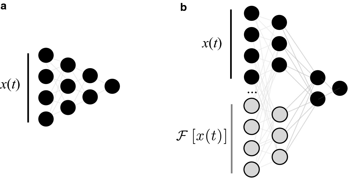
Transform raw data using known physics to create additional, more informative input features. {.fragment}
The model receives both raw measurements and physics-derived quantities. {.fragment}
No change to the model architecture — just better inputs. {.fragment}
This is the simplest form of physics-informed ML [@neuer2024machine]. {.fragment}
Classic network (left) vs FFT-enriched physics-informed network (right). The FT output is concatenated with raw data as additional input. [@neuer2024machine]
FFT-based enrichment
Compute the Fourier spectrum of time-series data. {.fragment}
Frequency-domain features capture periodicity, resonance frequencies, and harmonic content. {.fragment}
Particularly useful for vibration data, acoustic signals, and cyclic processes. {.fragment}
Implementation: np.fft.fft(signal) → magnitude and phase spectra as additional features. {.fragment}
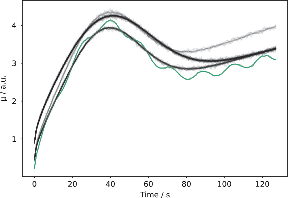
Motor current time series: “good” (black) vs “bad” (green, oscillating). FFT readily separates classes invisible to raw time-series models. [@neuer2024machine]
Wavelet-based enrichment
Wavelet transforms capture time-frequency information simultaneously. {.fragment}
Unlike FFT, wavelets localize both time and frequency — useful for transient phenomena. {.fragment}
Continuous wavelet transform (CWT) or discrete wavelet transform (DWT). {.fragment}
Application: detecting phase transitions in temperature-time curves. {.fragment}
Derivative-based enrichment
Compute numerical derivatives of input signals: {.fragment}
First derivative: rates of change (cooling rate, strain rate). {.fragment}
Second derivative: curvature, acceleration. {.fragment}
Derivatives encode dynamics that raw values do not capture. {.fragment}
Can also compute spatial gradients for field data. {.fragment}
Histogram and statistical enrichment
Compute histograms, moments, or percentiles of input distributions. {.fragment}
Summarize variability within a measurement window. {.fragment}
Example: instead of raw vibration signal, provide mean, std, skewness, kurtosis, and percentiles. {.fragment}
Reduces dimensionality while preserving statistical information. {.fragment}
Captures dominant variation patterns as compact features. {.fragment}
The PCA components have physical interpretation (e.g., baseline, peak shape, noise). {.fragment}
Combine with raw peak features for a rich input representation. {.fragment}
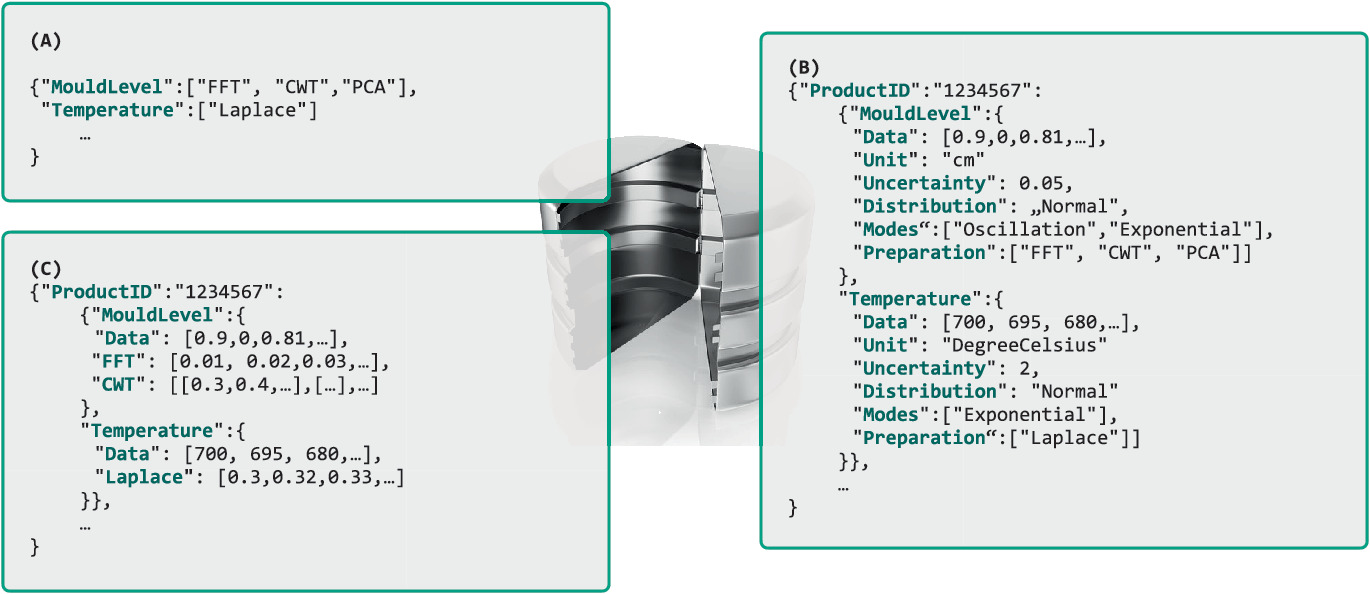
Expert knowledge objects
Domain experts specify transformations based on physical understanding: {.fragment}
Dimensionless groups (Reynolds number, Nusselt number). {.fragment}
Known functional relationships (Arrhenius equation for temperature dependence). {.fragment}
Physical units and scaling. {.fragment}
These “expert knowledge objects” are formalized as input transformations [@neuer2024machine]. {.fragment}
Data table linking variables to their recommended physical transformations — a practical implementation of expert knowledge objects. [@neuer2024machine]
Checkpoint: data enrichment design
Scenario: Your raw features are temperature vs time for a cooling process.
For PINNs, we also need \(f_{} / \) — derivatives w.r.t. inputs.
Both are computed by the same auto-diff machinery.
Using auto-diff for physics constraints
Key insight: auto-diff can compute any derivative of the NN output w.r.t. any input variable.
\(f / t\), \(^2 f / ^2\), \(f\) — all available at no extra modeling effort.
These derivatives are exact (up to floating-point precision), not finite differences.
This enables evaluating PDE residuals within the training loop.
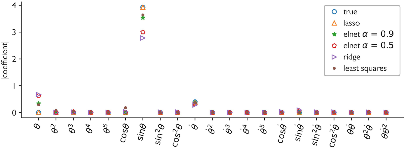
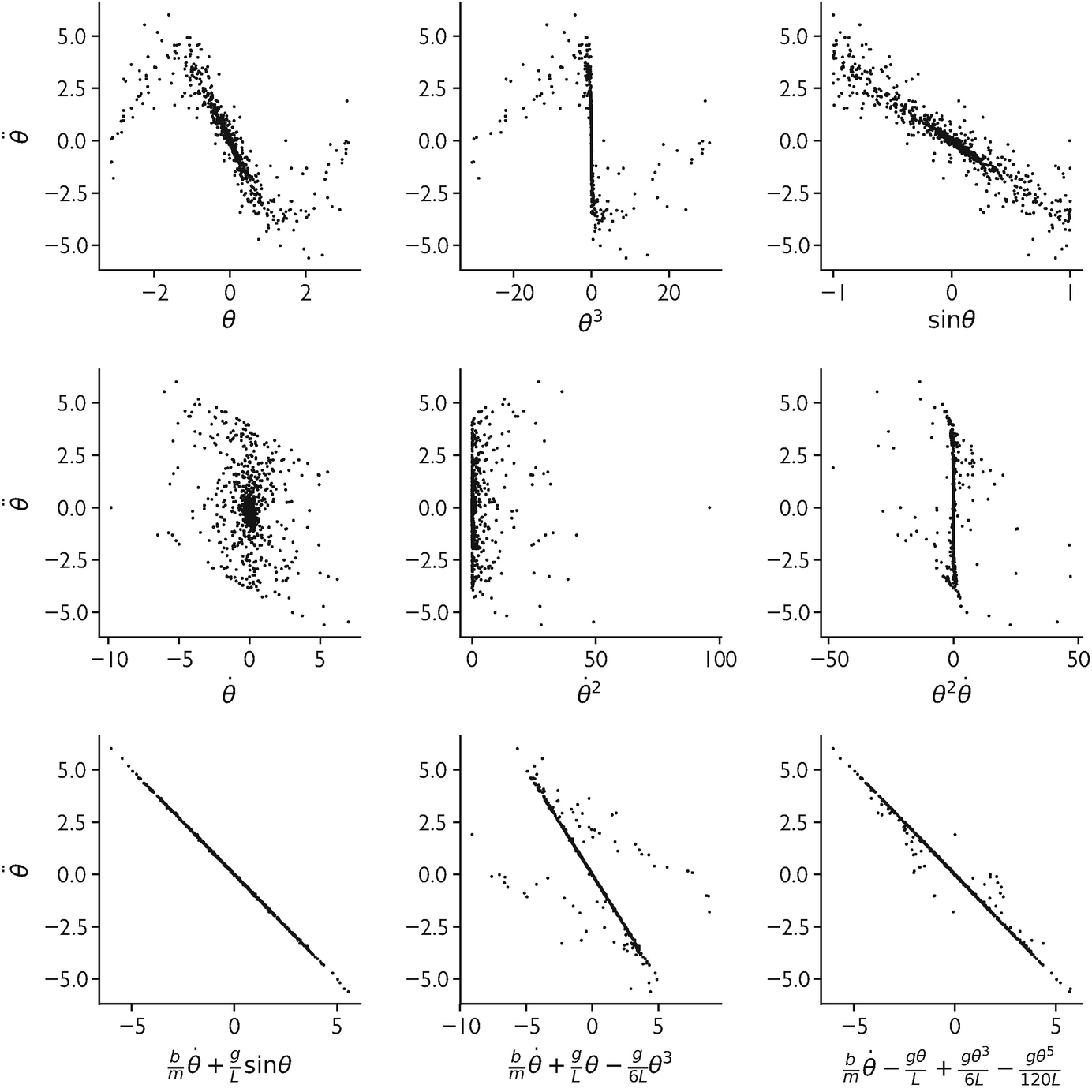
Equation discovery: scatter of pendulum acceleration against candidate dictionary terms. Lasso regression identifies the two true terms (\(\), \(\)) and zeros out the rest. [@mcclarren2021machine]
\(\) is the residual of the governing equation (PDE, ODE, conservation law).
Evaluated at \(M\) collocation points sampled across the domain.
No labels needed for physics loss — just the equation.
Collocation points
Points in the domain where the physics residual is evaluated.
Typically sampled uniformly or according to an adaptive strategy.
More collocation points → better physics enforcement but higher cost.
Collocation points do not need observed data — they provide physics supervision for free.
Scatter plots of pendulum acceleration against candidate dictionary terms. The true governing equation emerges from sparse data — analogous to evaluating physics residuals at collocation points. [@mcclarren2021machine]
The role of lambda
\(\) balances data fit vs physics compliance:
\(= 0\): pure data-driven (standard NN).
\(\): pure physics (NN solves the PDE).
Intermediate \(\): compromise between data and physics.
The optimal \(\) depends on data quality, physics accuracy, and problem specifics.
Choosing lambda
Too high: model satisfies physics perfectly but ignores noisy data → underfitting data.
Too low: model fits data well but violates physics → physically inconsistent predictions.
Adaptive strategies: adjust \(\) during training based on relative magnitudes of \(J_{}\) and \(J_{}\).
Cross-validation on held-out data can also guide \(\) selection.
PINN architecture
Typically a standard fully-connected NN (MLP) with smooth activations (tanh, swish).
Inputs: spatial coordinates \(\) and/or time \(t\).
Output: physical field values (temperature, velocity, stress).
Auto-diff is used to compute all required derivatives within the loss function.
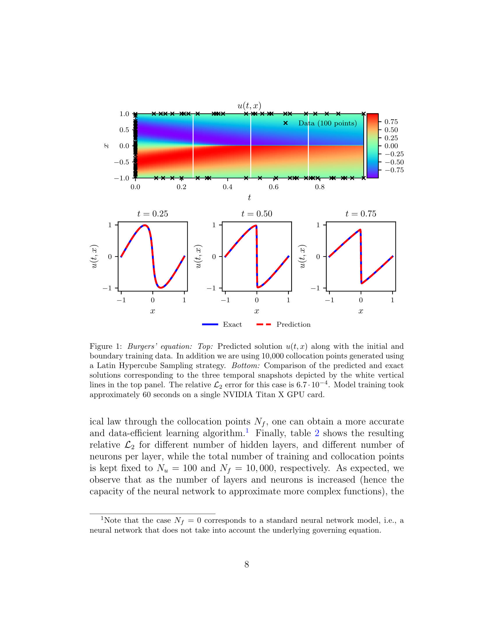
Figure: predicted Burgers field (top) matches exact solution at three time slices (bottom) — trained with only 100 data points [@raissi2019physics].
Raissi et al. (2019) Fig. 1: PINN solution of the Burgers equation. Top: predicted spatio-temporal field with 100 training points (×). Bottom: exact (blue) vs PINN prediction (red) at \(t=0.25, 0.50, 0.75\). [@raissi2019physics]
Checkpoint: PINN loss design
Problem: Heat diffusion \( = \) with noisy temperature measurements.
Data loss: \(J_{} = i (T_i^{} - f{}(_i, t_i))^2\).
Guaranteed Consistency: BCs are met even before training starts.
Search Space: Restricts the model to physically plausible functions.
Reference: @lagaris1998artificial.
Lagaris substitution: example
Problem: \(f(\mathbf{0}) = a\), general ODE/PDE on \([0, L]\).
Trial solution: \(f(\mathbf{x}) = a + \mathbf{x} \cdot \text{NN}(\mathbf{x})\).
At \(\mathbf{x} = \mathbf{0}\): \(f(\mathbf{0}) = a + \mathbf{0} \cdot \text{NN}(\mathbf{0}) = a\) ✓ (regardless of NN).
The NN learns the deviation from the initial condition.
For \(f(\mathbf{0})=a, f(L)=b\): \(f(\mathbf{x}) = a + \frac{\mathbf{x}}{L}(b-a) + \mathbf{x}(L-\mathbf{x})\text{NN}(\mathbf{x})\).
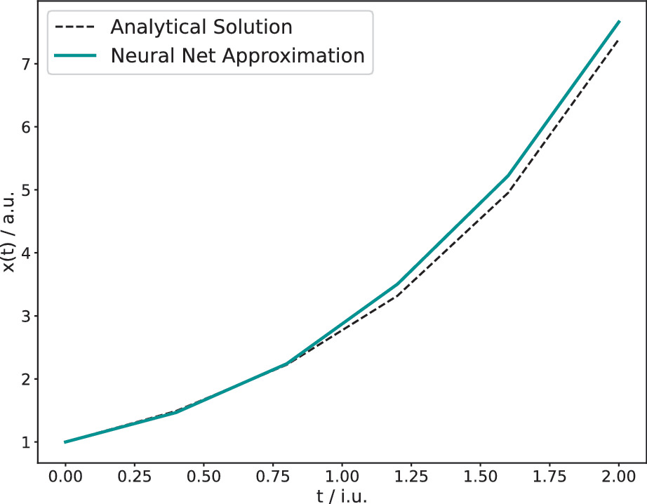
Lagaris for ODE: \(\mathbf{x}' = \mathbf{x}\), \(\mathbf{x}(0) = \mathbf{1}\)
Trial solution: \(\mathbf{x}(t) = \mathbf{1} + t \cdot \text{NN}(t)\).
IC: \(\mathbf{x}(0) = \mathbf{1}\) ✓.
ODE residual: \(\mathcal{R} = \mathbf{x}'(t) - \mathbf{x}(t) = \text{NN}(t) + t \cdot \text{NN}'(t) - \mathbf{1} - t \cdot \text{NN}(t)\).
Minimize \(\sum_j \mathcal{R}(t_j)^2\) over collocation points.
Exact solution: \(\mathbf{x}(t) = e^t \mathbf{1}\). The NN should learn \(\text{NN}(t) \approx (e^t - 1)\mathbf{1}/t\).
Analytical solution \(e^t\) (black) vs neural network solution (green) for \(x’=x\), \(x(0)=1\). The Lagaris substitution guarantees the IC and the NN learns the remaining shape. [@neuer2024machine]
Advantages of hard enforcement
BCs are exactly satisfied — no penalty term, no violation, no tuning.
Reduces the search space: the NN only learns the unknown part of the solution.
Fewer hyperparameters (no \(_{}\)).
Often leads to faster convergence and better solutions.
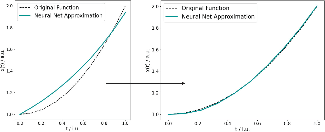
Neural integrators and ODE solvers
Use a NN to parameterize the solution of an ODE.
Train by minimizing the ODE residual at collocation points.
The NN produces a continuous, differentiable solution — no time-stepping discretization.
Advantage: solution at any point \(t\) without marching through time steps.
NN solution converging to the analytical integral (parabola). Left: early training (loss > 1.5). Right: converged solution (loss < 0.02). [@neuer2024machine]
Checkpoint: Lagaris design
Problem: \(f’’() = g()\), \(f() = \), \(f() = \).
Trial solution: \(f() = (-) ()\).
Check: \(f() = () = \) ✓. \(f() = () = \) ✓.
The NN freely shapes the solution in the interior while BCs are guaranteed.
Occam’s razor and model selection
Occam’s razor: among models that explain the data equally well, prefer the simplest.
Physics constraints simplify the model by restricting the hypothesis space.
A physics-constrained model with 100 parameters may be effectively simpler than an unconstrained model with 10.
Connects to the effective number of parameters (Unit 12).
Information-theoretic perspective
Minimum Description Length (MDL): the best model minimizes total description length = model complexity + data residual.
Physics priors reduce the model complexity term — less needs to be learned from data.
This provides a formal justification for why physics-informed models generalize better.
Small-data advantage of PINNs
With only 10 labeled data points, a PINN enforcing the governing ODE can outperform a standard NN trained on 1000 points.
The physics residual provides supervision at every collocation point — effectively unlimited “free data.”
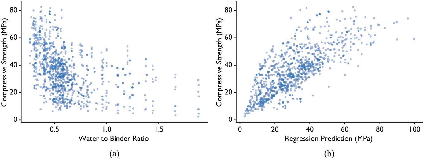
Physics feature engineering also exploits domain knowledge: water/binder ratio is a derived physical variable that substantially improves concrete strength prediction. {.fragment}
Concrete compressive strength vs water/binder ratio (a physics-derived feature) and regression model output. Adding this domain variable improves \(R^2\) from 0.800 to 0.834. [@mcclarren2021machine]
Explainability benefit
Physics-constrained models are more interpretable:
The model respects known laws by design — no surprising violations.
\(\lambda\) quantifies the data-physics tradeoff.
Residual analysis reveals where the model deviates from physics.
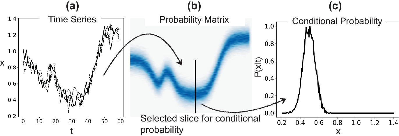
Process corridors: model the expected probability distribution of a process signal; points outside the corridor flag anomalies. {.fragment}
2D probability corridor for time series. The shaded band encodes the normal process distribution; measurements outside it (red circles) are flagged as anomalies. [@neuer2024machine]
Limitations: when PINNs fail
Incorrect physics: if the governing equation is wrong, the PINN converges to a wrong solution.
Multi-scale problems: features at very different scales (e.g., boundary layers) cause conflicting gradients.
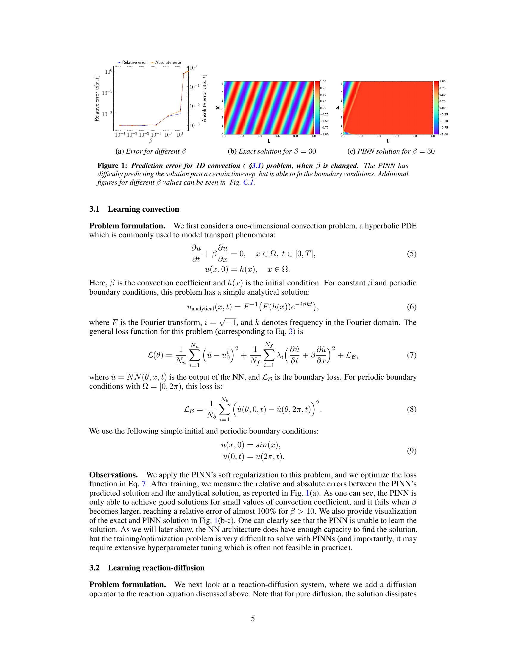
Convection-dominated PDEs: PINN error increases sharply with the convection coefficient \(\beta\) — standard soft-constraint training fails for large \(\beta\)[@krishnapriyan2021characterizing].
Krishnapriyan et al. (2021) Fig. 1: PINN failure on the 1D convection equation. (a) Prediction error vs \(\beta\); (b) exact solution for \(\beta=30\); (c) PINN solution for \(\beta=30\) — the network cannot learn the sharp advecting front. [@krishnapriyan2021characterizing]
Limitations: optimization challenges
Balancing \(J_{}\) and \(J_{}\) is notoriously difficult.
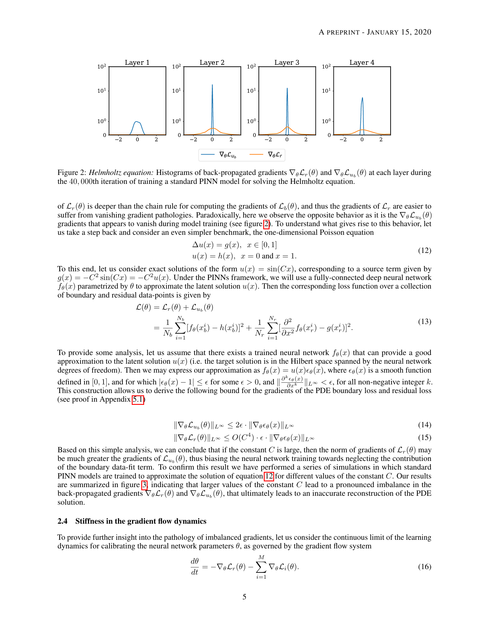
Gradient imbalance: gradients of \(J_{\text{physics}}\) (orange) dominate those of \(J_{\text{data}}\) (blue) by orders of magnitude — the network ignores boundary conditions [@wang2021understanding]. {.fragment}
Stiff PDEs cause training instability — physics-loss gradients can be very large. {.fragment}
Active area of research: improved architectures, training strategies, and adaptive \(\lambda\)[@wang2021understanding]. {.fragment}
Wang et al. (2021) Fig. 2: Back-propagated gradient histograms at each hidden layer for a PINN solving the Helmholtz equation. Gradients from \(\nabla_\theta \mathcal{L}_u\) (data, blue) are orders of magnitude smaller than those from \(\nabla_\theta \mathcal{L}_r\) (physics, orange) — a root cause of PINN training failure. [@wang2021understanding]
Limitations: computational cost
Auto-diff through PDE residuals requires computing high-order derivatives — expensive.
Each training step evaluates physics at \(M\) collocation points — cost scales with domain size.
For complex 3D problems, PINNs can be slower than traditional solvers.
PINNs are most competitive when data is very scarce or when inverse problems are solved.
Beyond PINNs: architectural constraints
Equivariant networks: build symmetries (rotation, translation) into the architecture.
Hamiltonian NNs: parameterize the Hamiltonian; dynamics automatically conserve energy.
Neural operators (DeepONet, FNO): learn mappings between function spaces.
These embed physics more deeply than loss-based constraints.
DeepONet: learning operators between function spaces
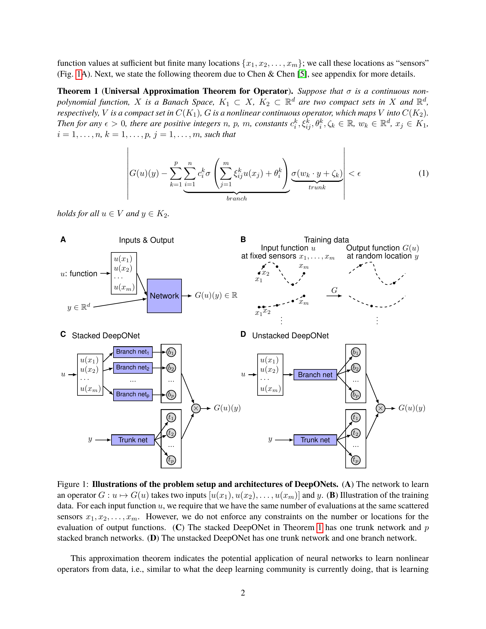
Standard NNs map vectors to vectors. DeepONet maps functions to functions: \(G: u \mapsto G(u)\)[@lu2021learning]. {.fragment}
Branch net: encodes the input function \(u\) sampled at fixed sensor locations. {.fragment}
Trunk net: encodes the query location \(y\) where the output is evaluated. {.fragment}
Output: \(G(u)(y) = \sum_k b_k(u) \cdot t_k(y)\) — a learned dot product of branch and trunk embeddings. {.fragment}
Application: PDE solution operators (given an initial condition \(u\), predict the solution field at any later time). {.fragment}
Lu et al. (2021) Fig. 1: DeepONet architectures. (A) Network for operator \(G\). (B) Training data: input function \(u\) at sensors \(x_1,\ldots,x_m\), output \(G(u)(y)\) at random \(y\). (C) Stacked and (D) unstacked variants with branch and trunk networks. [@lu2021learning]
Fourier Neural Operator (FNO)
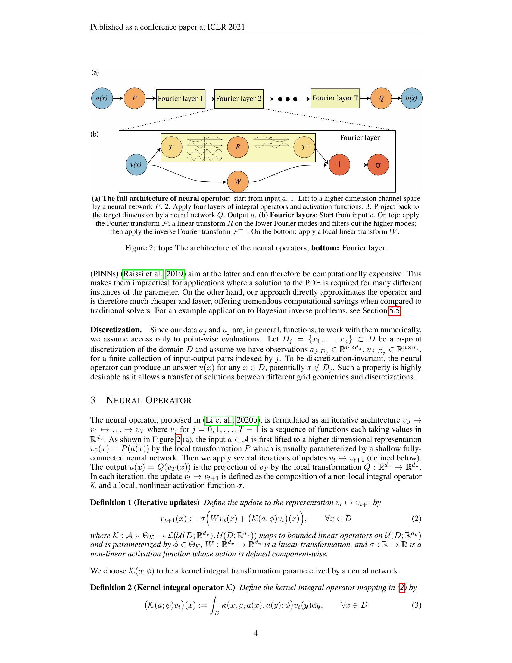
FNO learns PDE solution operators by parameterizing the convolution in Fourier space[@li2020fourier]. {.fragment}
Spectral convolution: lift input to higher-dim representation → apply learned weights to low Fourier modes → transform back. {.fragment}
Resolution-invariant: trained at one resolution, evaluated at another. {.fragment}
State-of-the-art for Navier–Stokes, Darcy flow, and weather prediction. {.fragment}
Key advantage over PINN: inference is a single forward pass (no per-instance optimization). {.fragment}
Li et al. (2020) Fig. 2: Top — Full FNO architecture: input lifted by \(P\), passed through \(T\) Fourier layers, projected by \(Q\). Bottom — One Fourier layer: spectral conv (left branch, keeps low-frequency modes) + local linear transform (right branch), summed and activated. [@li2020fourier]
Beyond FNO
PINO[@li2024pino] — pairs FNO’s operator output with a PINN-style physics-residual loss. Closes the data-vs-physics trade-off: FNO learns from data, PINN enforces physics; PINO does both.
GNN-based PDE solvers (MeshGraphNets, [@pfaff2021mgn]) — for unstructured meshes where FNO’s regular-grid FFT doesn’t apply. Encode the simulation mesh as a graph; message-passing replaces convolution. Currently the standard for industrial CFD / fluid surrogates.
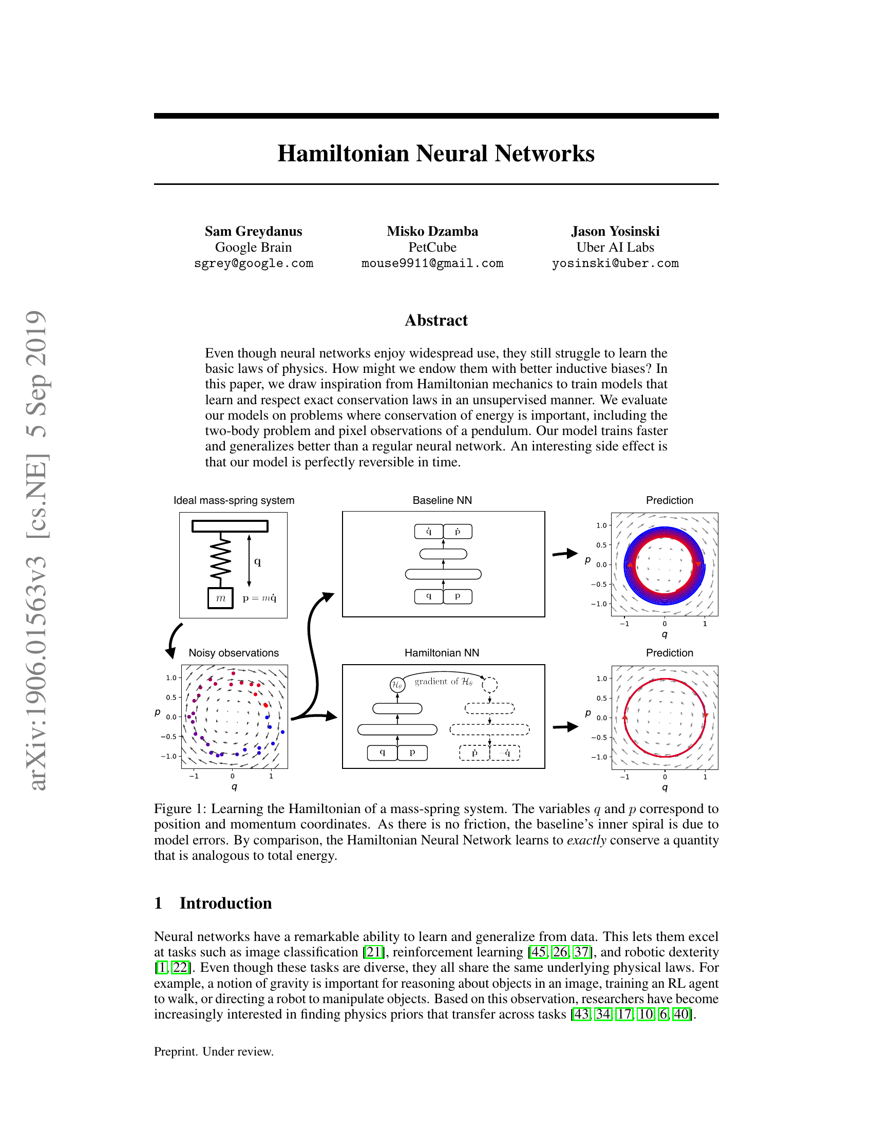
Hamiltonian Neural Networks (HNN)
A vanilla NN predicts the next state of a dynamical system; energy is not conserved by construction. {.fragment}
HNN[@greydanus2019hamiltonian] learns the scalar Hamiltonian \(\mathcal{H}(q,p)\); equations of motion follow from: {.fragment}
This guarantees energy conservation by the structure of the network, not by penalty. {.fragment}
Baseline NN spirals inward (violates conservation); HNN stays on the correct orbit. {.fragment}
Greydanus et al. (2019) Fig. 1: Mass-spring system. Top row: ideal system and baseline NN prediction (inner spiral — energy loss). Bottom row: noisy observations and HNN prediction (correct circular orbit — energy conserved). [@greydanus2019hamiltonian]
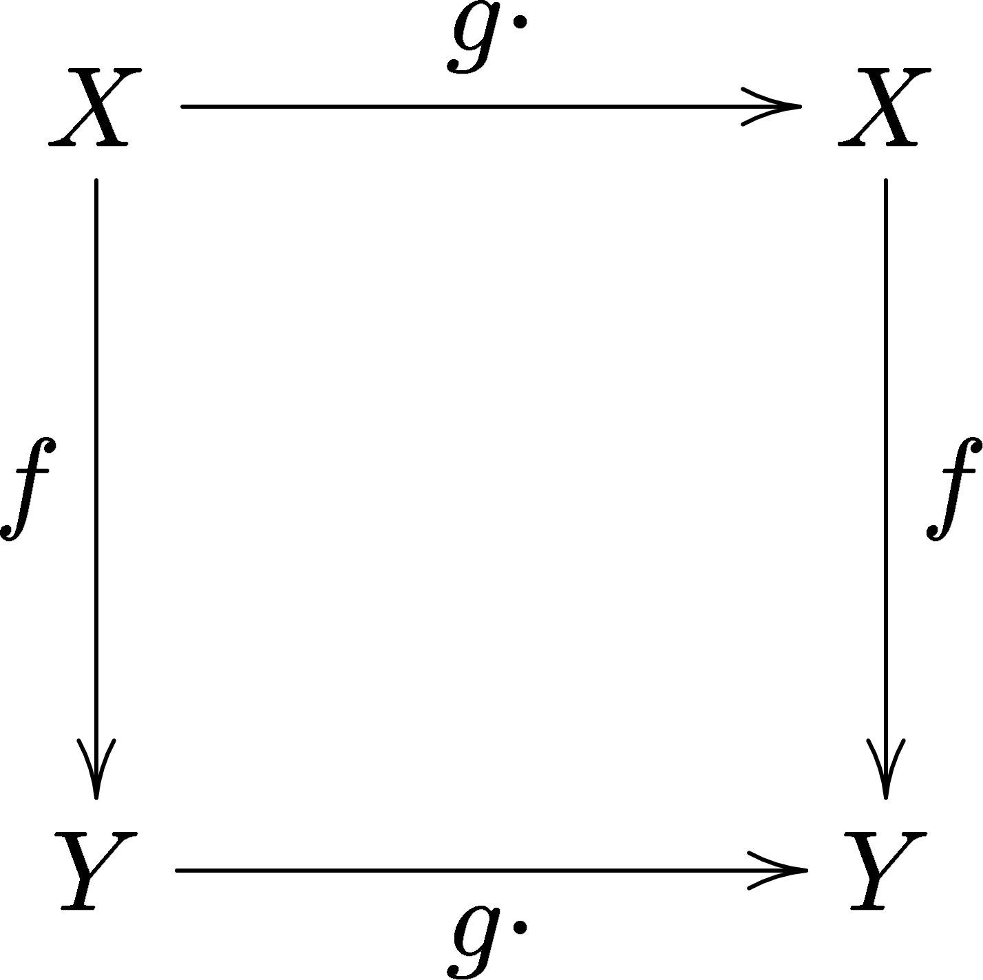
Group-equivariant neural networks
A function \(f: X \to Y\) is equivariant to a group \(G\) if applying a symmetry \(g \in G\) before or after \(f\) gives the same result [@cohen2016group]: {.fragment}
\[f(g \cdot x) = g \cdot f(x)\]
Standard CNNs are equivariant to translation. G-CNNs extend this to rotations, reflections, and other symmetry groups. {.fragment}
Applications: molecular property prediction (rotational symmetry of atoms), crystallography, medical image segmentation. {.fragment}
Key benefit: fewer parameters needed — symmetry-related outputs are tied by the group structure, not learned independently. {.fragment}
Commutative diagram defining equivariance: applying the group action \(g\cdot\) in the input space \(X\) then mapping by \(f\) gives the same result as mapping first then applying \(g\cdot\) in the output space \(Y\). (Wikimedia Commons, CC-BY-SA 3.0, David Benbennick 2005)