Mathematical Foundations of AI & ML
Appendix: Algorithm Compendium

Prof. Dr. Philipp Pelz

FAU Erlangen-Nürnberg

How to use this deck

One slide per algorithm:
- Input/Output header, numbered steps
- One line why it works
- One classic pitfall
Notation follows the lectures:
\(\boldsymbol{\theta}, \mathbf{w}\) parameters, \(\eta\) learning rate, \(\lambda\) regularization weight, \(\nabla\) gradient, \(\sigma(\cdot)\) activation.
The unit tag on each slide points to the lecture with the full derivation and context.
Exam bar: Be able to write each of these from memory and state the pitfall.

Unit	Algorithms
1	data splitting & k-fold CV
2	OLS/ridge, PCA via SVD
3	GD/SGD, Newton, logistic regression
4	MLP forward, backprop, 2D convolution
5	k-means, EM for GMM, autoencoder
6	momentum/Nesterov, AdaGrad
7	MLE/MAP
8	CART, random forest, gradient boosting, permutation importance
9	t-SNE, UMAP, SimCLR
10	attention, multi-head, transformer block, ViT
11	VAE, DDPM training, sampling + guidance
12	GP regression, ensembles/MC dropout, calibration, EI
13	PINN, Lagaris
14	sensitivity analysis

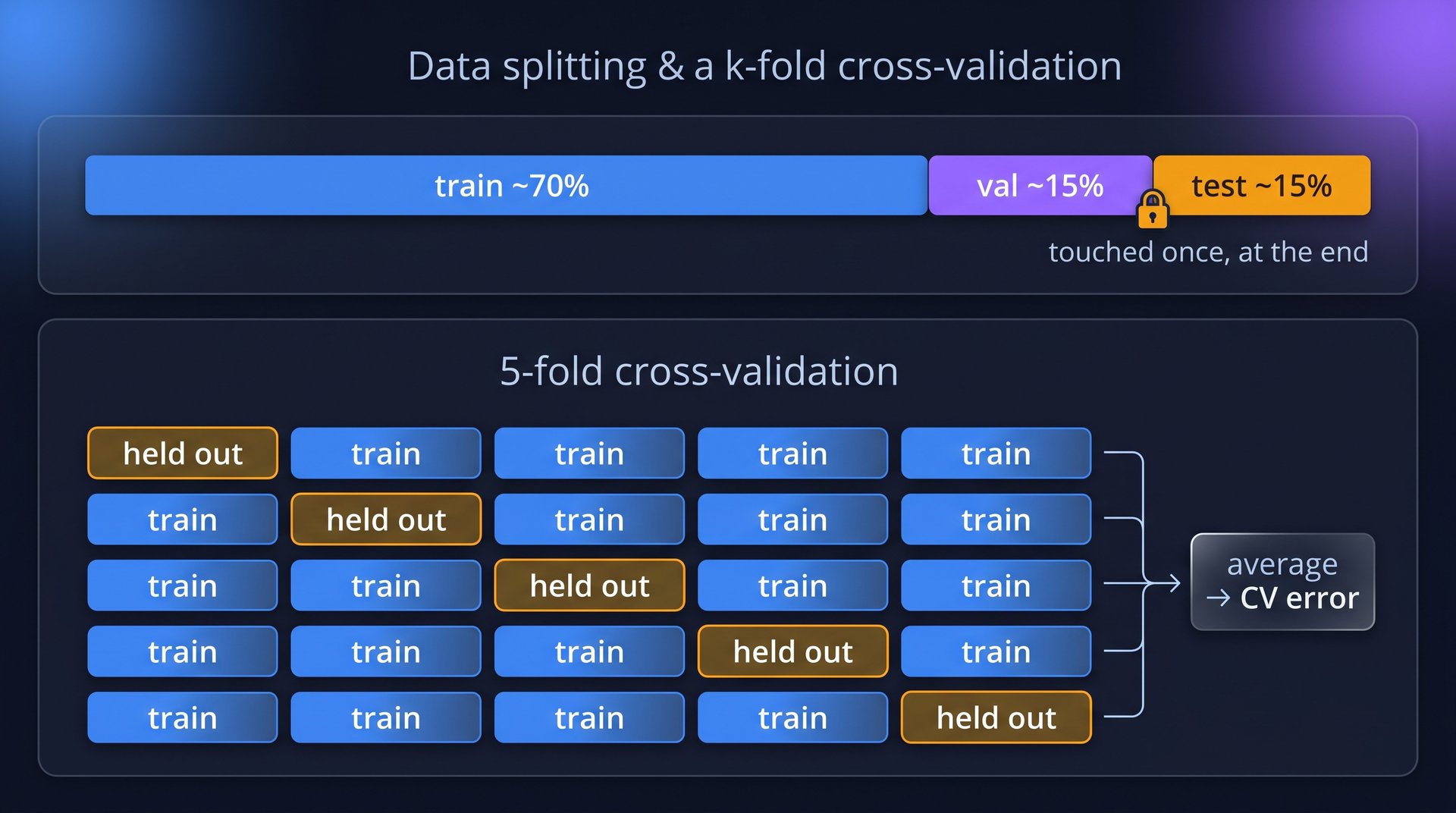
Data splitting & k-fold cross-validation — Unit 1

Input:  dataset D of N samples, model family, fold count k
Output: honest generalization estimate; final model

Train/val/test protocol:
1:  split D into train (~70%), val (~15%), test (~15%)   # once, first
2:  fit candidate models on train
3:  select hyperparameters by val score
4:  report test score ONCE, at the very end

k-fold cross-validation:
1:  partition D into k equal folds D₁ … D_k
2:  for j = 1 … k do
3:      train on D \ D_j;   e_j ← score on held-out D_j
4:  end for
5:  return CV error (1/k) Σ_j e_j

Why it works: every point is validated exactly once — a low-variance estimate from limited data.
Pitfall: preprocessing fitted on all of D (scaling, PCA, feature selection) leaks the test set — fit it inside each fold.

Data splitting & k-fold CV — overview figure

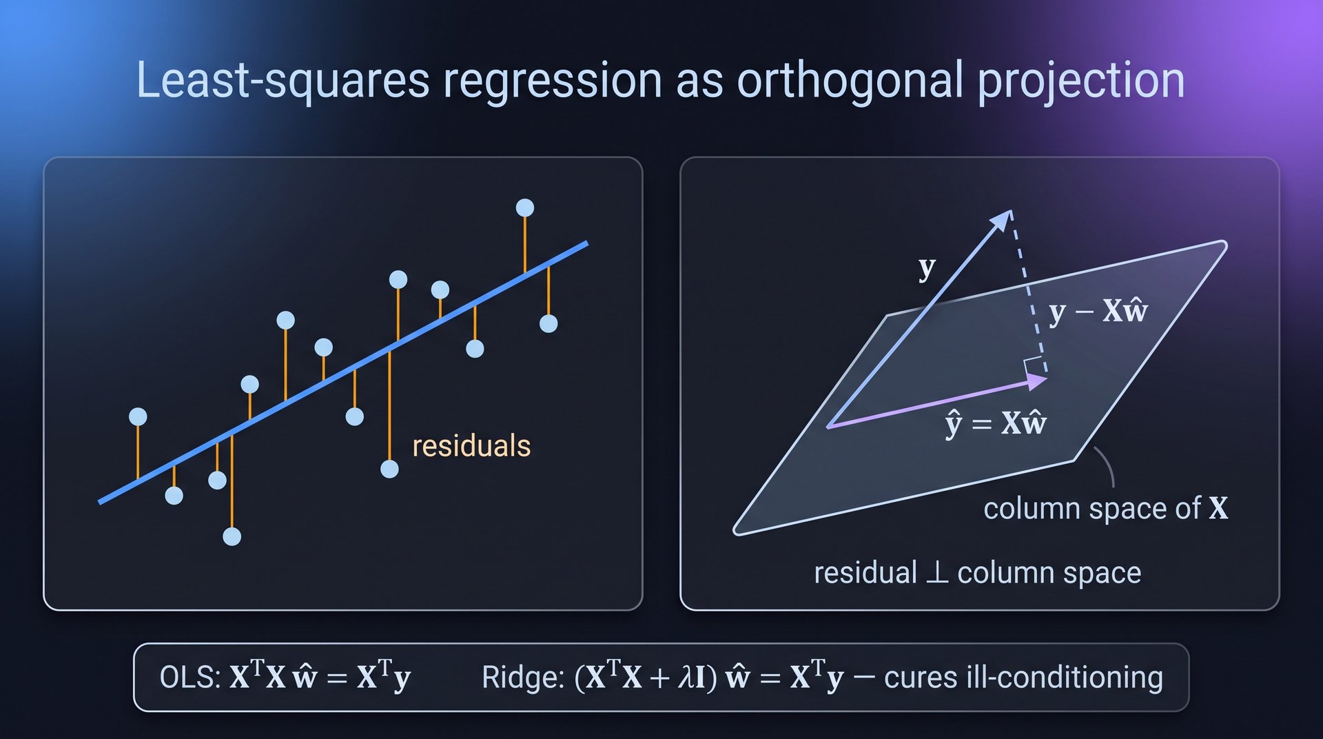
Ordinary least squares (+ ridge) — Unit 2

Input:  design matrix X ∈ ℝ^{N×D}, targets y ∈ ℝ^N
Output: weights ŵ

1:  G ← XᵀX;   b ← Xᵀy
2:  solve G ŵ = b                    # Cholesky; never invert explicitly
3:  return ŵ                         # ŵ = (XᵀX)⁻¹Xᵀy

Ridge variant:     solve (XᵀX + λI) ŵ = Xᵀy      # λ > 0 cures ill-conditioning
Basis expansion:   replace X by Φ, Φ_ij = φ_j(xᵢ)  # same equations,
                                                   # nonlinear in x, linear in w

Why it works: orthogonality — the residual \(\mathbf{y} - \mathbf{X}\hat{\mathbf{w}}\) is perpendicular to the column space of \(\mathbf{X}\).
Pitfall: near-collinear columns make \(\mathbf{X}^T\mathbf{X}\) ill-conditioned — use ridge or the SVD pseudo-inverse.

OLS + ridge — overview figure

PCA via SVD — Unit 2

Input:  data X ∈ ℝ^{N×D}, target dimension k
Output: components V_k, scores Z, explained variance

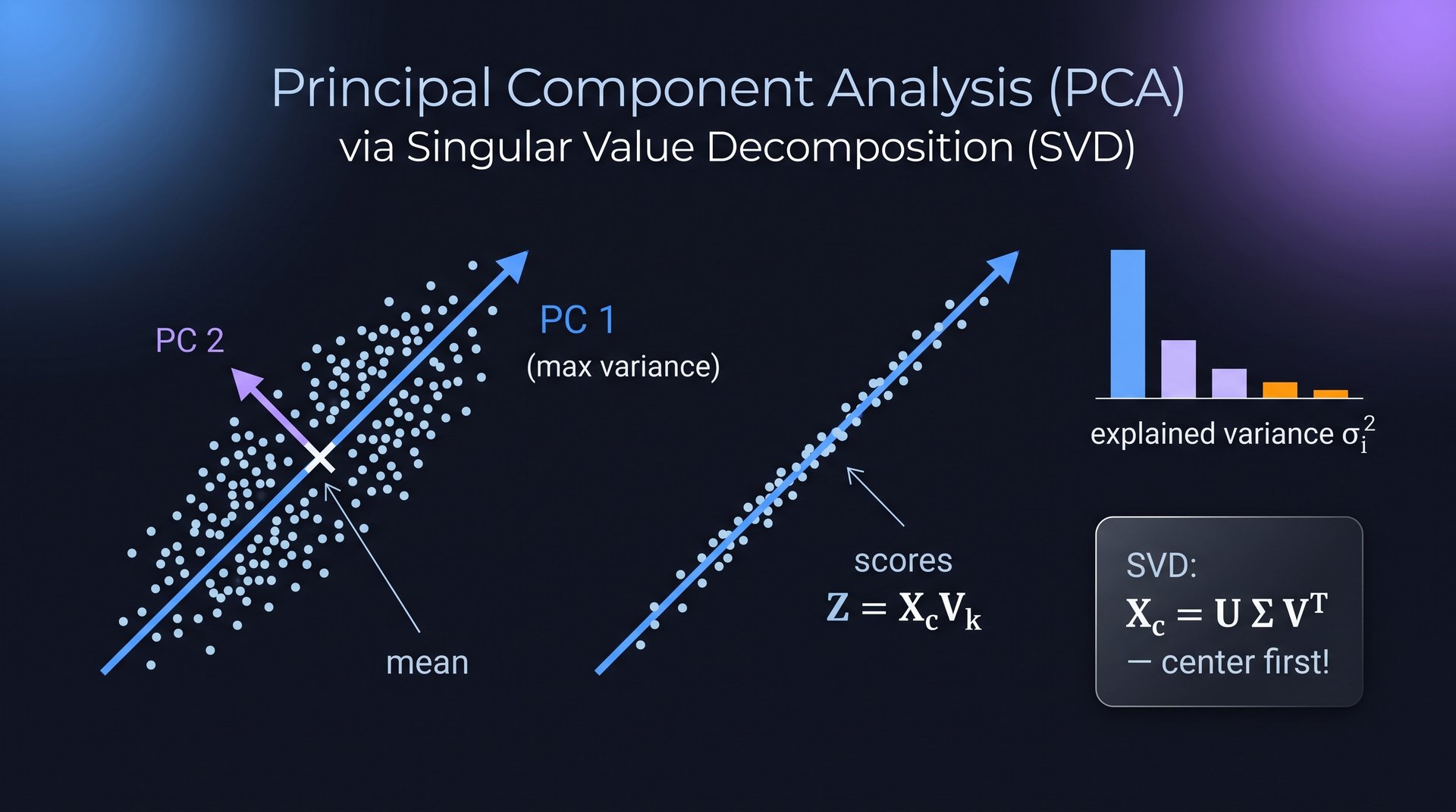
1:  x̄ ← column means;   X_c ← X − 1x̄ᵀ            # CENTER first
2:  U, Σ, Vᵀ ← SVD(X_c)                            # σ₁ ≥ σ₂ ≥ …
3:  V_k ← first k columns of V                      # principal components
4:  Z ← X_c V_k                                     # k-dim scores
5:  explained variance of PC i:  σᵢ²/(N−1);  ratio σᵢ²/Σ_j σ_j²
6:  return V_k, Z

Rank-k approximation (Eckart–Young):  X_k ← U_k Σ_k V_kᵀ
    # best possible ‖X_c − A‖_F over all rank-k matrices → denoising

Why it works: columns of \(\mathbf{V}\) are eigenvectors of the covariance \(\mathbf{S} = \mathbf{X}_c^T\mathbf{X}_c/(N{-}1)\) — the directions of maximal variance.
Pitfall: forgetting to center (PC 1 then points at the mean); fit PCA on training data only.

PCA via SVD — overview figure

Gradient descent, SGD, minibatch — Unit 3

Input:  loss L(w) = (1/N) Σᵢ Lᵢ(w), init w₀, learning rate η, steps T
Output: trained weights w

1:  w ← w₀
2:  for t = 1 … T do
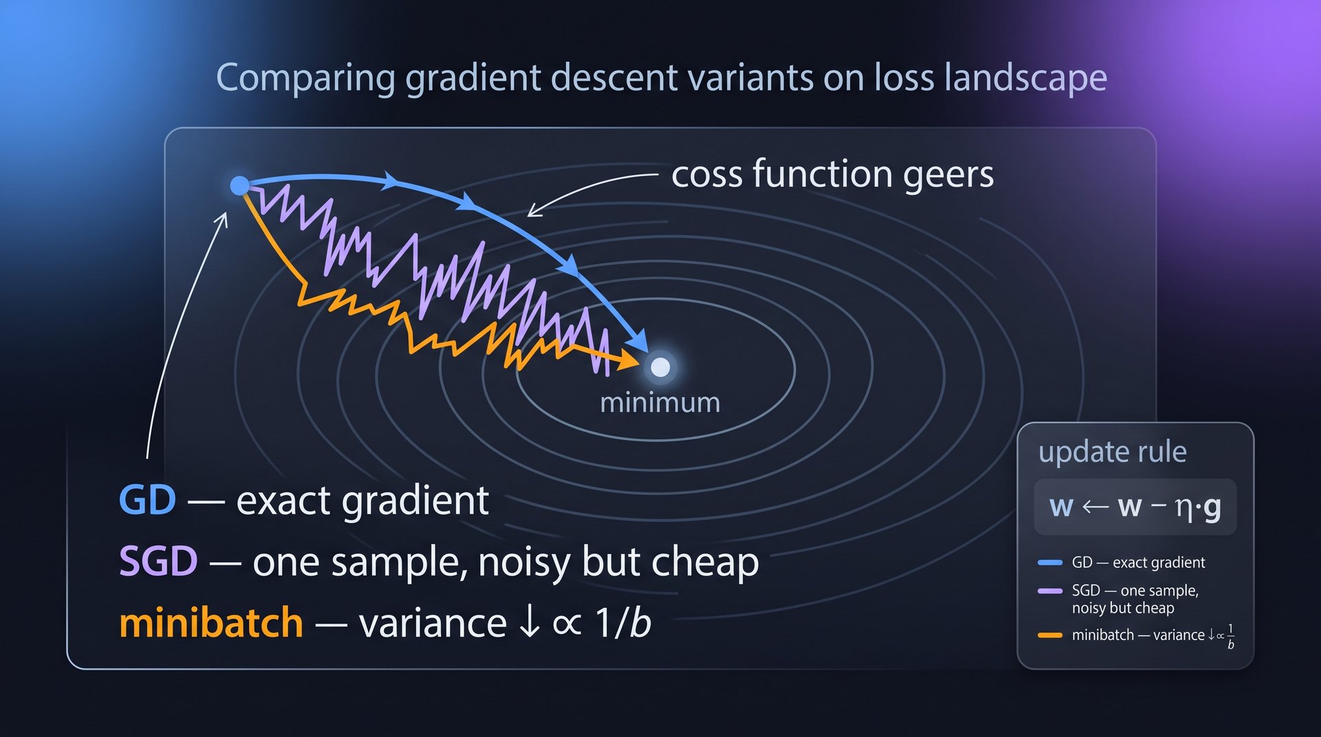
3:      (GD)         g ← ∇L(w)                        # exact, one pass over N
4:      (SGD)        g ← ∇Lᵢ(w),  i ~ Uniform{1…N}    # unbiased: 𝔼[g] = ∇L
5:      (minibatch)  g ← (1/b) Σ_{i∈B_t} ∇Lᵢ(w)       # variance ↓ ∝ 1/b, GPU-friendly
6:      w ← w − η · g
7:  end for
8:  return w

Why it works: for small \(\eta\), the first-order Taylor expansion gives \(L(\mathbf{w} - \eta\nabla L) \approx L(\mathbf{w}) - \eta\|\nabla L\|^2 < L(\mathbf{w})\).
Pitfall: \(\eta\) too large diverges or oscillates, too small crawls — read the loss curve before anything else.

GD / SGD / minibatch — overview figure

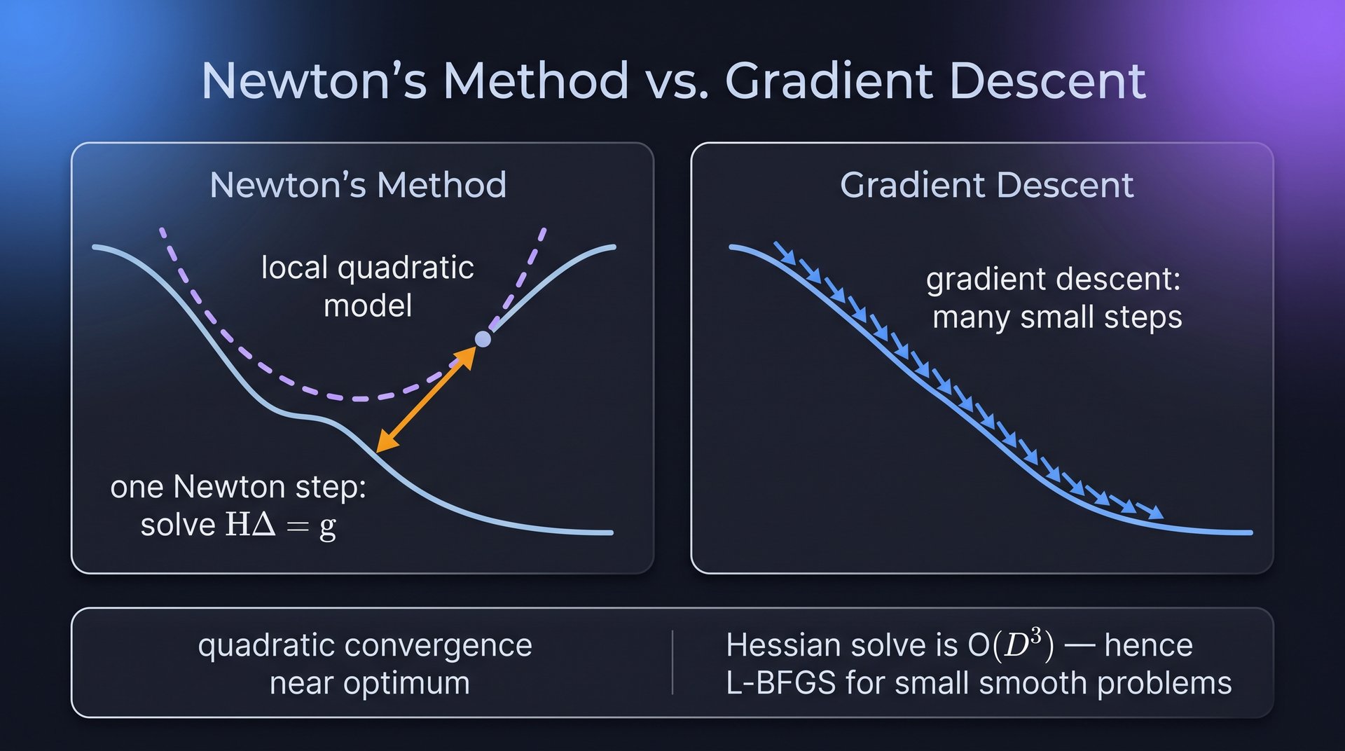
Newton’s method — Unit 3

Input:  loss f(w), init w₀, tolerance ε
Output: w near a stationary point

1:  w ← w₀
2:  repeat
3:      g ← ∇f(w);   H ← ∇²f(w)          # Hessian, D×D
4:      solve H Δ = g                     # O(D³)
5:      w ← w − Δ
6:  until ‖g‖ < ε

Quasi-Newton (BFGS / L-BFGS): approximate H⁻¹ from steps s_t = w_{t+1}−w_t
and gradient differences y_t = ∇f_{t+1}−∇f_t — no Hessian ever formed.

Why it works: minimizes the local quadratic model exactly — one step on quadratics, quadratic convergence near the optimum.
Pitfall: \(O(D^3)\) and indefinite Hessians rule it out for deep nets — that is why L-BFGS lives on small/smooth problems (e.g. PINNs, GP hyperparameters).

Newton’s method — overview figure

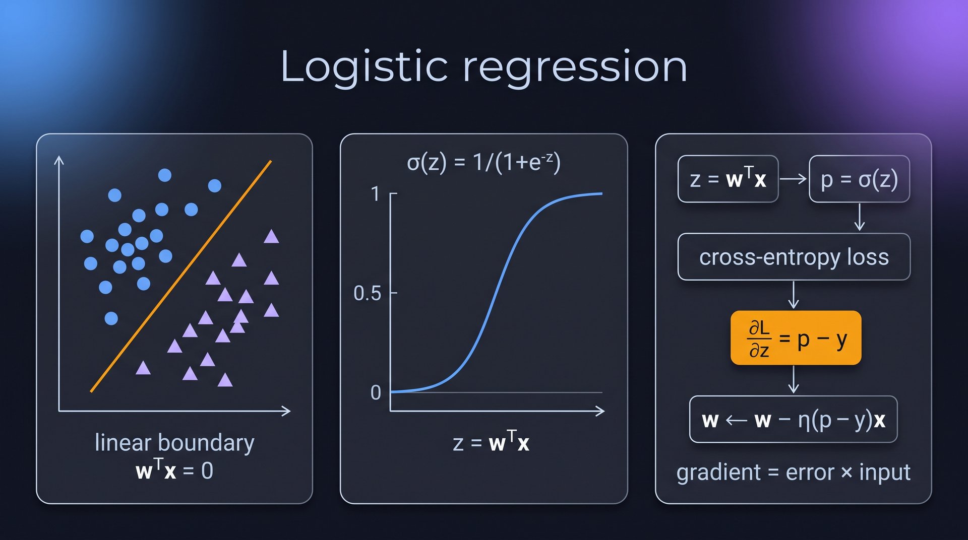
Logistic regression training — Unit 3

Input:  data {(xᵢ, yᵢ)}, yᵢ ∈ {0,1}, init w, learning rate η
Output: weights w for p(y=1|x) = σ(wᵀx)

1:  repeat over (minibatches of) samples i:
2:      zᵢ ← wᵀxᵢ;    pᵢ ← σ(zᵢ) = 1/(1+e^{−zᵢ})
3:      L ← −[ yᵢ log pᵢ + (1−yᵢ) log(1−pᵢ) ]     # cross-entropy = Bernoulli NLL
4:      ∂L/∂zᵢ = pᵢ − yᵢ                           # the famous simplification
5:      w ← w − η (pᵢ − yᵢ) xᵢ
6:  until converged

Multi-class:  softmax ŷ_c = exp(o_c)/Σ_j exp(o_j);   L = −Σ_c y_c log ŷ_c

Why it works: the loss is the NLL of the Bernoulli noise model, so the gradient is simply error × input.
Pitfall: using MSE on probabilities instead of cross-entropy — gradients vanish exactly at confident wrong answers.

Logistic regression — overview figure

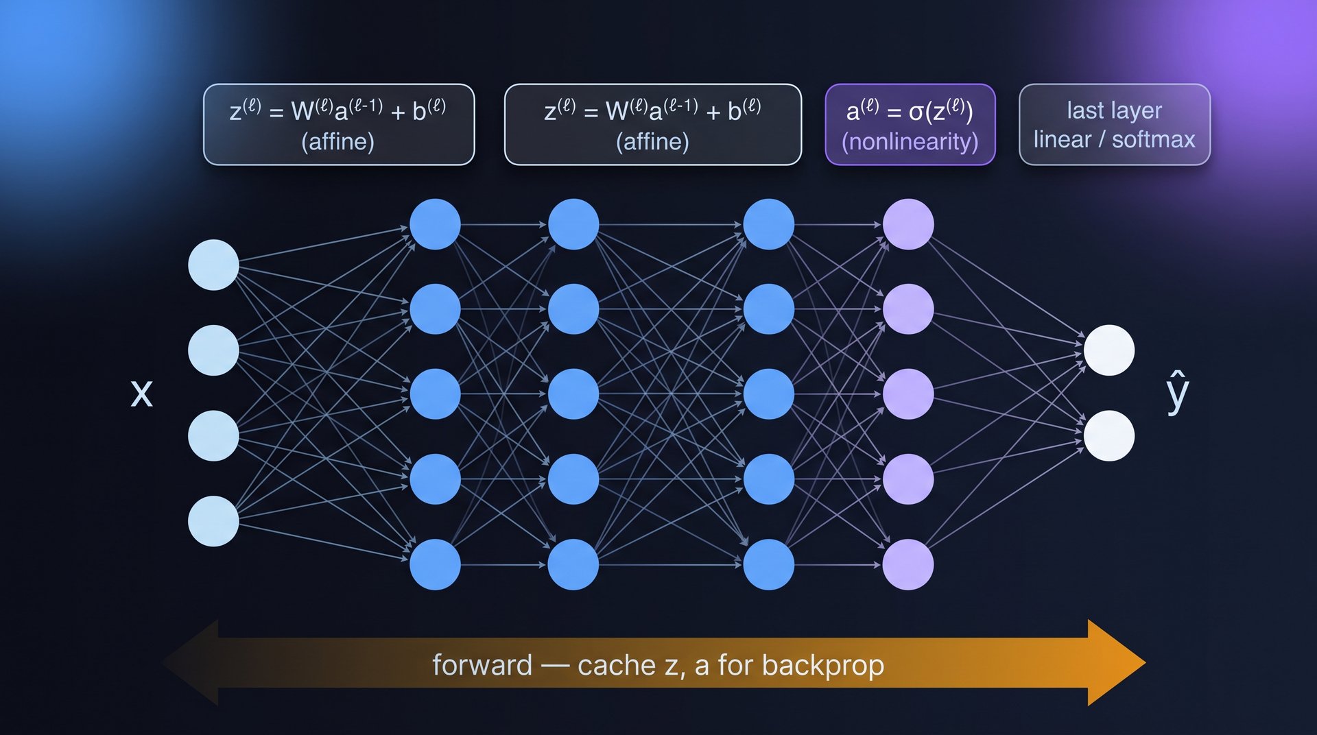
MLP forward pass — Unit 4

Input:  x ∈ ℝ^D, layers ℓ = 1…L with W⁽ℓ⁾, b⁽ℓ⁾, activation σ
Output: prediction ŷ (+ cache for backprop)

1:  a⁽⁰⁾ ← x
2:  for ℓ = 1 … L−1 do
3:      z⁽ℓ⁾ ← W⁽ℓ⁾ a⁽ℓ⁻¹⁾ + b⁽ℓ⁾        # affine;  W⁽ℓ⁾ ∈ ℝ^{M_ℓ × M_{ℓ−1}}
4:      a⁽ℓ⁾ ← σ(z⁽ℓ⁾)                    # elementwise nonlinearity
5:  end for
6:  ŷ ← W⁽L⁾ a⁽L⁻¹⁾ + b⁽L⁾               # last layer linear (or softmax)
7:  return ŷ;  cache all z⁽ℓ⁾, a⁽ℓ⁾

Why it works: alternating affine + nonlinear maps is a universal approximator; without \(\sigma\) the whole stack collapses to one linear map.
Pitfall: shape errors — track \(M_\ell \times M_{\ell-1}\) at every layer, batch dimension last or first but consistently.

MLP forward pass — overview figure

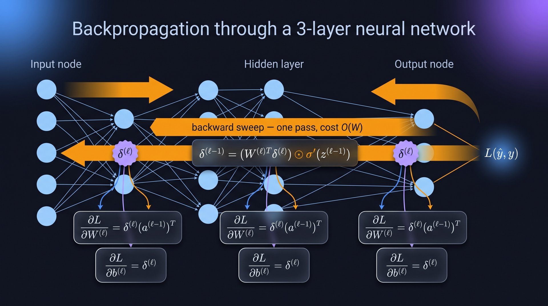
Backpropagation — Unit 4

Input:  cached forward pass (z⁽ℓ⁾, a⁽ℓ⁾), loss L(ŷ, y)
Output: gradients ∂L/∂W⁽ℓ⁾, ∂L/∂b⁽ℓ⁾ for all ℓ

1:  δ⁽L⁾ ← ∂L/∂ŷ                           # e.g. ŷ − y for MSE and CE+softmax
2:  for ℓ = L … 1 do                        # single backward sweep
3:      ∂L/∂W⁽ℓ⁾ ← δ⁽ℓ⁾ (a⁽ℓ⁻¹⁾)ᵀ
4:      ∂L/∂b⁽ℓ⁾ ← δ⁽ℓ⁾
5:      δ⁽ℓ⁻¹⁾ ← (W⁽ℓ⁾ᵀ δ⁽ℓ⁾) ⊙ σ′(z⁽ℓ⁻¹⁾)   # chain rule through layer ℓ
6:  end for

Why it works: the chain rule evaluated once and reused for every parameter — cost \(O(W)\), the same order as the forward pass (exam: not \(O(W^2)\)).
Pitfall: dropping the \(\odot\,\sigma'\) factor; for PINNs remember the same machinery also gives \(\partial f/\partial x\) — derivatives w.r.t. inputs.

Backpropagation — overview figure

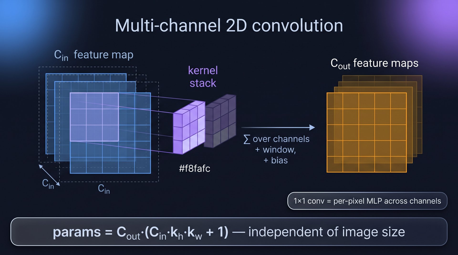
2D convolution (multi-channel) — Unit 4

Input:  X ∈ ℝ^{C_in×H×W}, kernels K ∈ ℝ^{C_out×C_in×k_h×k_w},
        bias b ∈ ℝ^{C_out}, padding p, stride s
Output: feature map H ∈ ℝ^{C_out×H_out×W_out}

1:  pad X with p zeros per side
2:  H_out ← ⌊(H + 2p − k_h)/s⌋ + 1        (W_out analogously)
3:  for each output channel d, each position (i, j):
4:      H_{d,i,j} ← b_d + Σ_c Σ_a Σ_b  K_{d,c,a,b} · X_{c, i·s+a, j·s+b}
5:  return H

Parameter count: C_out · (C_in · k_h · k_w + 1)    # independent of image size
1×1 convolution: mixes channels only — a per-pixel MLP

Why it works: a dense layer constrained by locality + weight sharing — translation equivariance and few parameters, matched to image statistics.
Pitfall: off-by-one in the output-shape formula; pooling/stride halve resolution — track shapes through the whole net.

2D convolution — overview figure

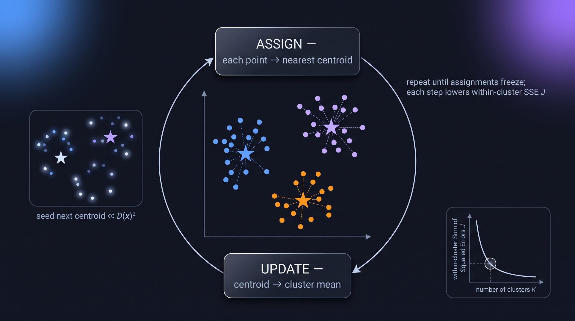
k-means (Lloyd + k-means++) — Unit 5

Input:  points {x₁ … x_N}, cluster count K
Output: centroids μ, assignments C

1:  # k-means++ initialization
2:  μ₁ ← random data point
3:  for k = 2 … K: pick μ_k = x with probability ∝ D(x)²
        # D(x) = distance to nearest already-chosen centroid
4:  repeat
5:      assign:  C_k ← {xᵢ : k = argmin_j ‖xᵢ − μ_j‖²}
6:      update:  μ_k ← (1/|C_k|) Σ_{xᵢ∈C_k} xᵢ
7:  until assignments unchanged
8:  return μ, C            # minimizes within-cluster SSE J … locally

Choosing K: elbow on J(K), or maximize mean silhouette s = (b−a)/max(a,b)

Why it works: coordinate descent on \(J\) — both steps can only decrease it, so it converges.
Pitfall: local optimum, init-dependent (use restarts), spherical clusters only — elongated or varying-density clusters break it.

k-means — overview figure

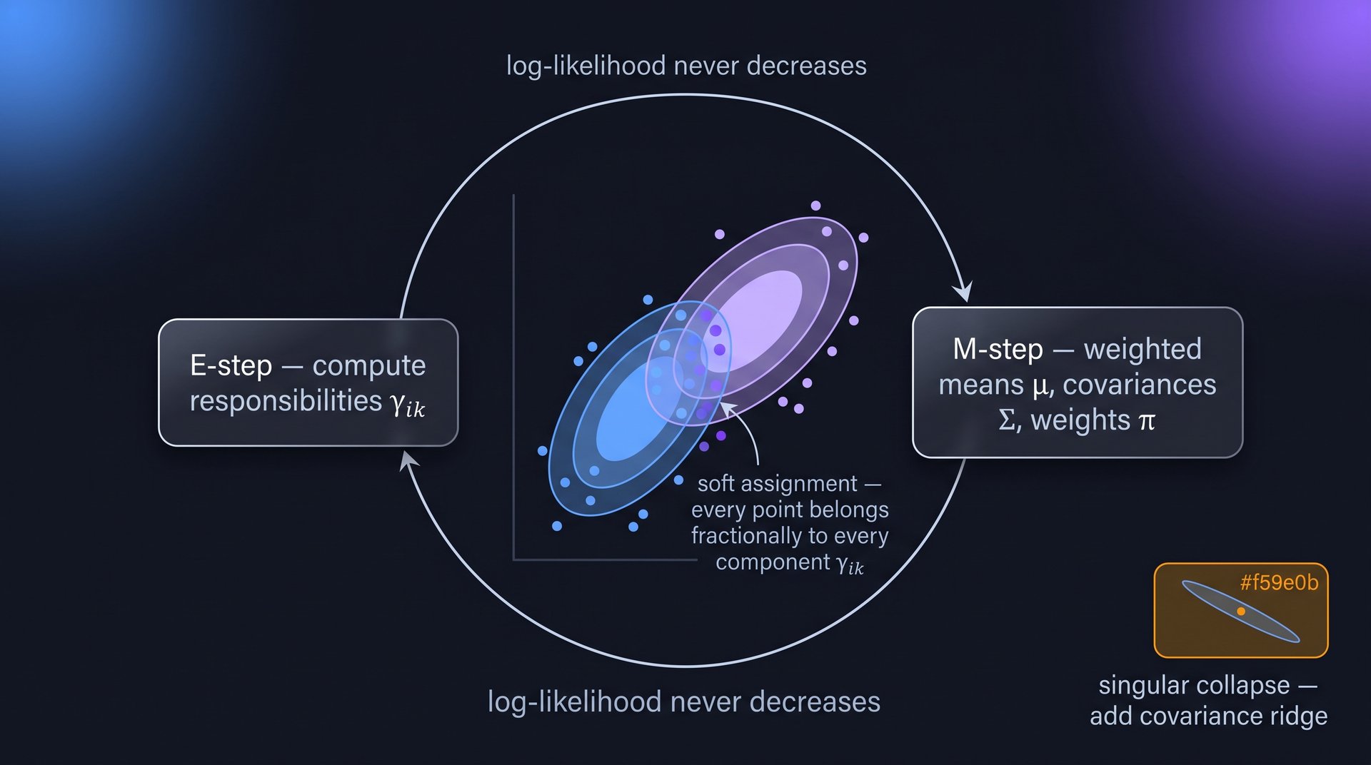
EM for Gaussian mixtures — Unit 5

Input:  data {xᵢ}, component count K (init means from k-means)
Output: weights π, means μ, covariances Σ

1:  repeat
2:      # E-step: responsibilities
3:      γᵢₖ ← π_k N(xᵢ; μ_k, Σ_k) / Σ_j π_j N(xᵢ; μ_j, Σ_j)
4:      # M-step: weighted updates, with N_k = Σᵢ γᵢₖ
5:      μ_k ← (1/N_k) Σᵢ γᵢₖ xᵢ
6:      Σ_k ← (1/N_k) Σᵢ γᵢₖ (xᵢ−μ_k)(xᵢ−μ_k)ᵀ
7:      π_k ← N_k / N
8:  until log-likelihood stops increasing     # guaranteed non-decreasing

Choosing K: minimize BIC(K) = −2 log p(D; θ̂_K) + p_K log N

Why it works: each E+M cycle is guaranteed not to decrease the data log-likelihood — soft k-means with covariances.
Pitfall: a component collapsing onto one point makes \(\Sigma_k\) singular — add a small ridge to the covariances.

EM for GMM — overview figure

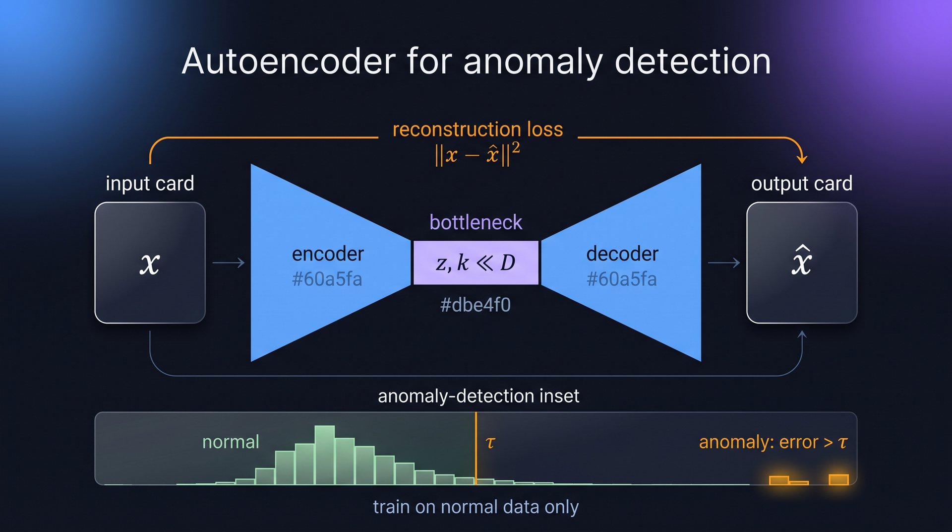
Autoencoder training + anomaly detection — Unit 5

Input:  data {xᵢ}, encoder f_φ, decoder g_θ, bottleneck dim k ≪ D
Output: trained φ, θ; anomaly detector

1:  repeat over minibatches
2:      z ← f_φ(x);    x̂ ← g_θ(z)
3:      L ← ‖x − x̂‖²                        # reconstruction loss
4:      gradient step on φ, θ
5:  until converged

Denoising variant:  feed x̃ = x + ε, still reconstruct the CLEAN x
Anomaly detection:  train on NORMAL data only;
    flag x if ‖x − g_θ(f_φ(x))‖² > τ        # τ = e.g. 99th percentile on train

Why it works: the bottleneck forces compression; a linear AE recovers exactly the PCA subspace — nonlinearity generalizes it to curved manifolds.
Pitfall: bottleneck too wide → the AE learns the identity and the codes are useless.

Autoencoder — overview figure

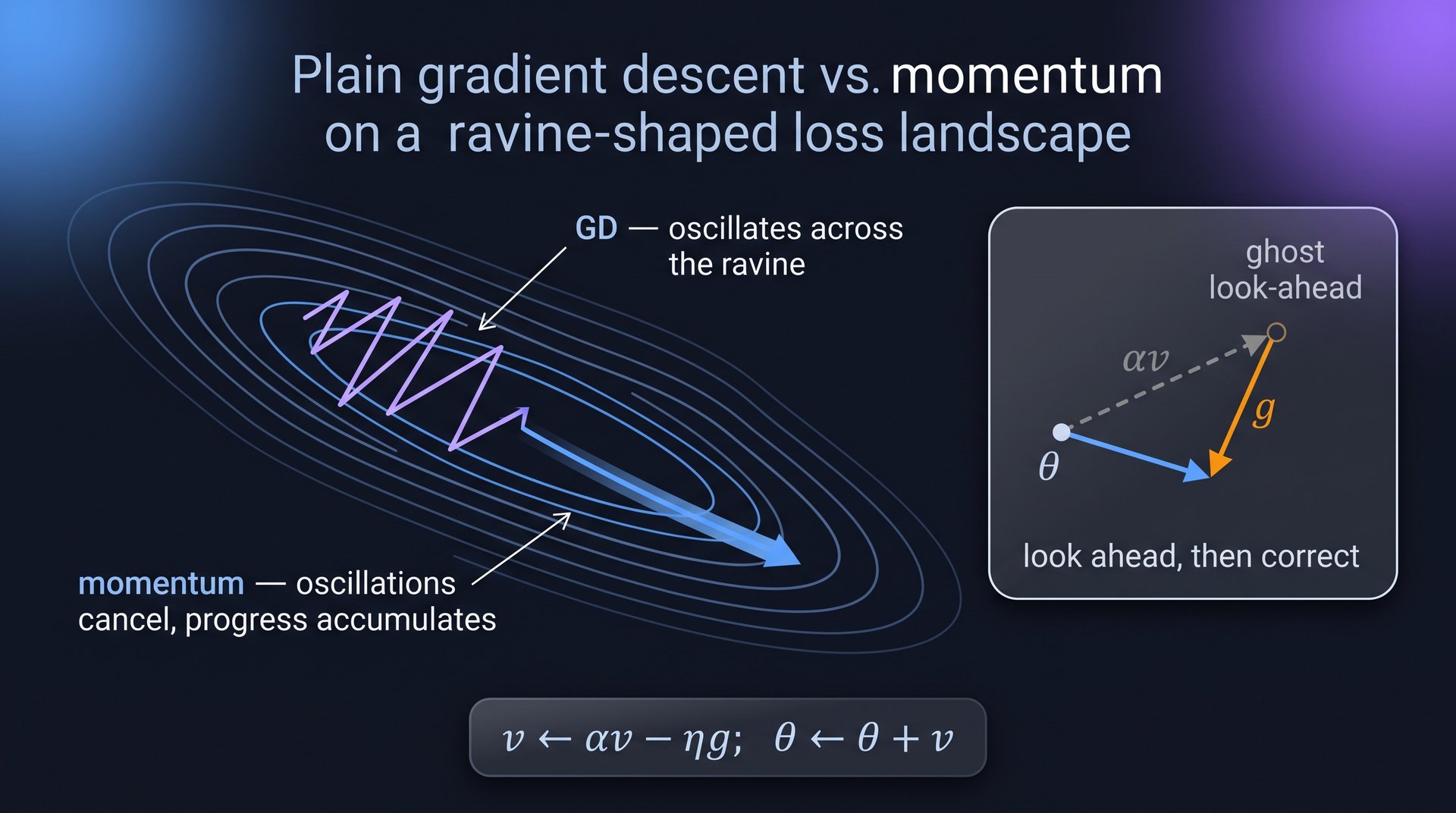
Momentum & Nesterov — Unit 6

Input:  gradients g⁽ᵗ⁾, learning rate η, momentum α (default 0.9)
Output: parameter trajectory θ⁽ᵗ⁾

Heavy ball:
1:  v⁽ᵗ⁺¹⁾ ← α v⁽ᵗ⁾ − η g⁽ᵗ⁾               # velocity accumulates history
2:  θ⁽ᵗ⁺¹⁾ ← θ⁽ᵗ⁾ + v⁽ᵗ⁺¹⁾

Nesterov (look-ahead):
1:  g̃ ← ∇L(θ⁽ᵗ⁾ + α v⁽ᵗ⁾)                  # gradient at the look-ahead point
2:  v⁽ᵗ⁺¹⁾ ← α v⁽ᵗ⁾ − η g̃
3:  θ⁽ᵗ⁺¹⁾ ← θ⁽ᵗ⁾ + v⁽ᵗ⁺¹⁾

Why it works: velocity averages recent gradients — oscillations across a ravine cancel, progress along the valley accumulates; Nesterov corrects before committing (\(O(1/t^2)\) convex rate vs \(O(1/t)\)).
Pitfall: \(\alpha\) and \(\eta\) interact — raising momentum without lowering the learning rate overshoots.

Momentum & Nesterov — overview figure

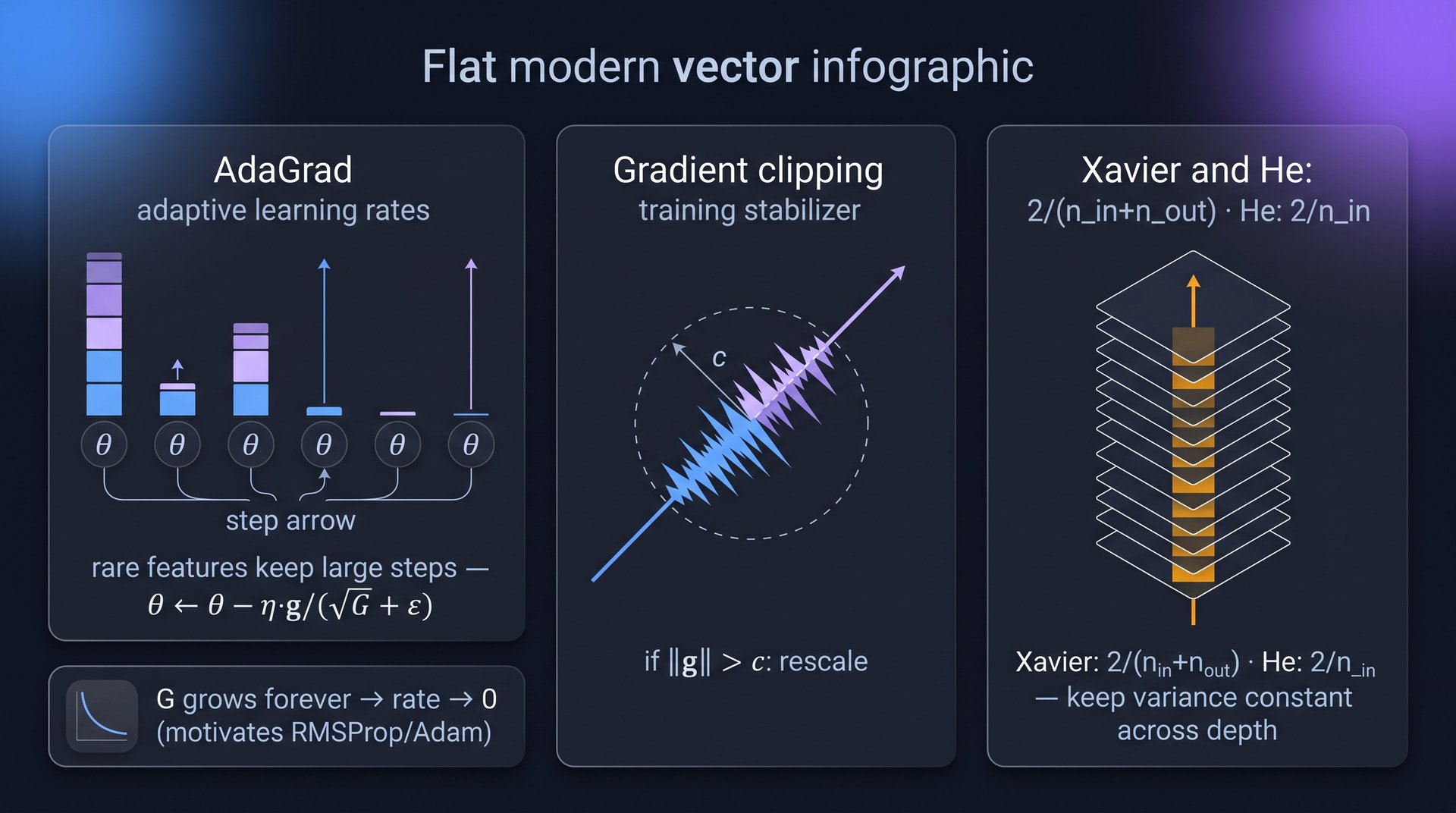
AdaGrad + training stabilizers — Unit 6

Input:  gradients g_t, global rate η, ε ≈ 1e−8
Output: per-parameter adapted updates

1:  G ← 0                                    # accumulator, same shape as θ
2:  for t = 1 … T do
3:      G ← G + g_t ⊙ g_t                    # accumulates forever
4:      θ ← θ − η · g_t / (√G + ε)           # elementwise adaptive rate
5:  end for

Stabilizer toolkit:
- gradient clipping:  if ‖g‖ > c:  g ← c · g/‖g‖         (c ≈ 1.0)
- init (keep variance constant across depth):
      Xavier  Var(W) = 2/(n_in + n_out)   for tanh/linear
      He      Var(W) = 2/n_in             for ReLU (factor 2: half the units die)

Why it works: parameters with rare/small gradients keep large effective learning rates — exactly the sparse-feature regime.
Pitfall: \(G\) grows monotonically so the rate decays to zero — the motivation for RMSProp/Adam’s moving average.

AdaGrad + stabilizers — overview figure

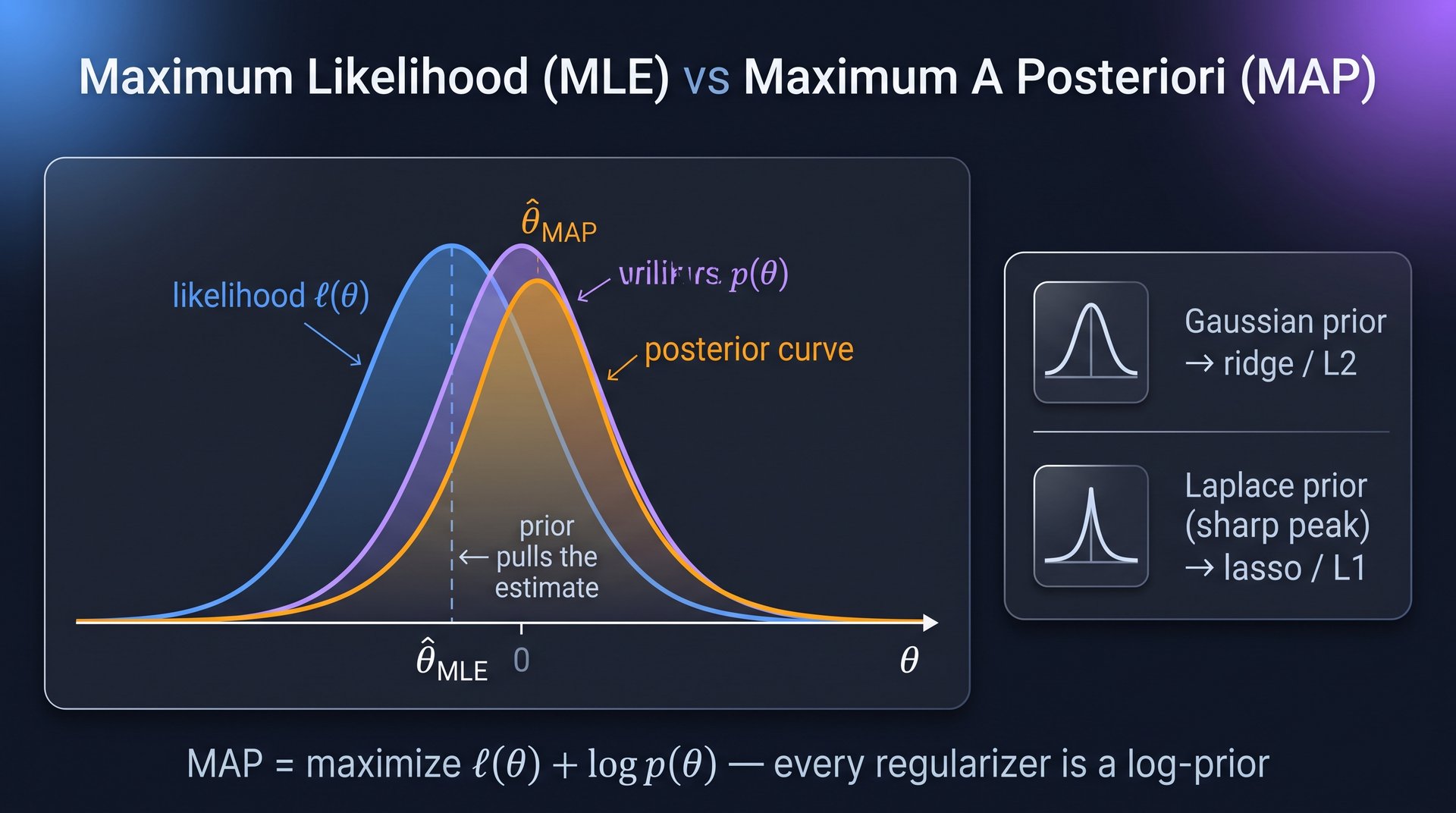
MLE and MAP estimation — Unit 7

Input:  data D = {xᵢ}, model p(x | θ)
Output: point estimate θ̂

1:  write the log-likelihood   ℓ(θ) = Σᵢ log p(xᵢ | θ)
2:  solve ∇_θ ℓ(θ) = 0 in closed form, or maximize numerically
3:  return θ̂_MLE

Gaussian example (closed form):
    μ̂ = (1/N) Σᵢ xᵢ;      σ̂² = (1/N) Σᵢ (xᵢ − μ̂)²

MAP variant:  maximize  ℓ(θ) + log p(θ)       # prior = regularizer
    Gaussian prior → ridge / L2;   Laplace prior → lasso / L1

Why it works: MSE minimization is Gaussian MLE; every regularizer is a log-prior — one framework unifies Units 1–3.
Pitfall: MLE overfits small \(N\) (e.g. \(\hat{\sigma}^2\) is biased) — exactly when the MAP prior earns its keep.

MLE & MAP — overview figure

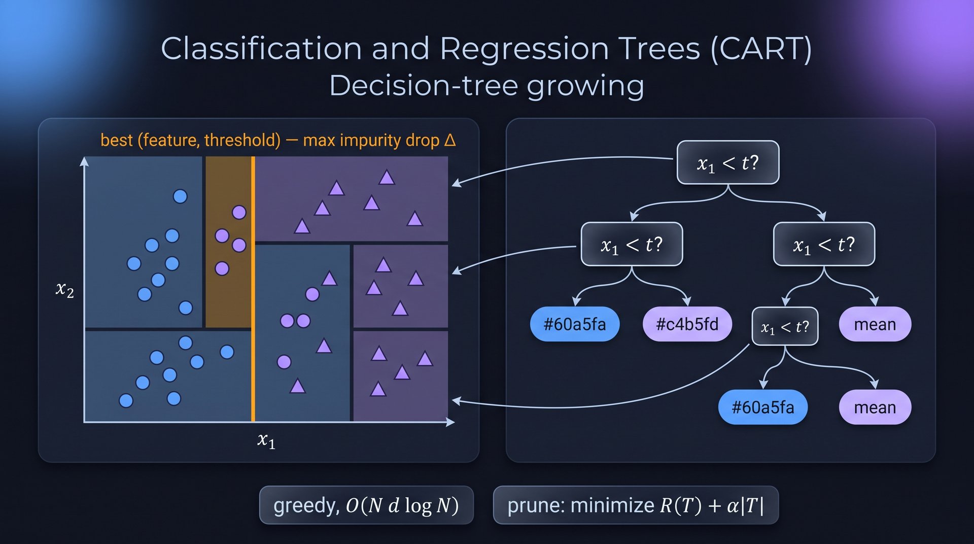
CART: growing a decision tree — Unit 8

Input:  node data, impurity I (variance | Gini | entropy), stopping rules
Output: decision tree

1:  if stopping rule met (max depth, min samples, no positive gain): make leaf
2:  for each feature j, each candidate threshold t:
3:      split into L, R
4:      Δ ← I(parent) − (N_L/N)·I(L) − (N_R/N)·I(R)     # impurity reduction
5:  keep the (j, t) with maximal Δ;  recurse on both children

Leaf prediction: mean y (regression) | majority class (classification)
Pruning: grow full, then minimize R(T) + α|T|, α chosen by CV

Why it works: greedy, loss-specific splits give a cheap (\(O(N d \log N)\)), interpretable, scale-invariant partition — no global optimization is attempted.
Pitfall: a single unpruned tree is a high-variance memorizer — that is the entire reason ensembles exist.

CART — overview figure

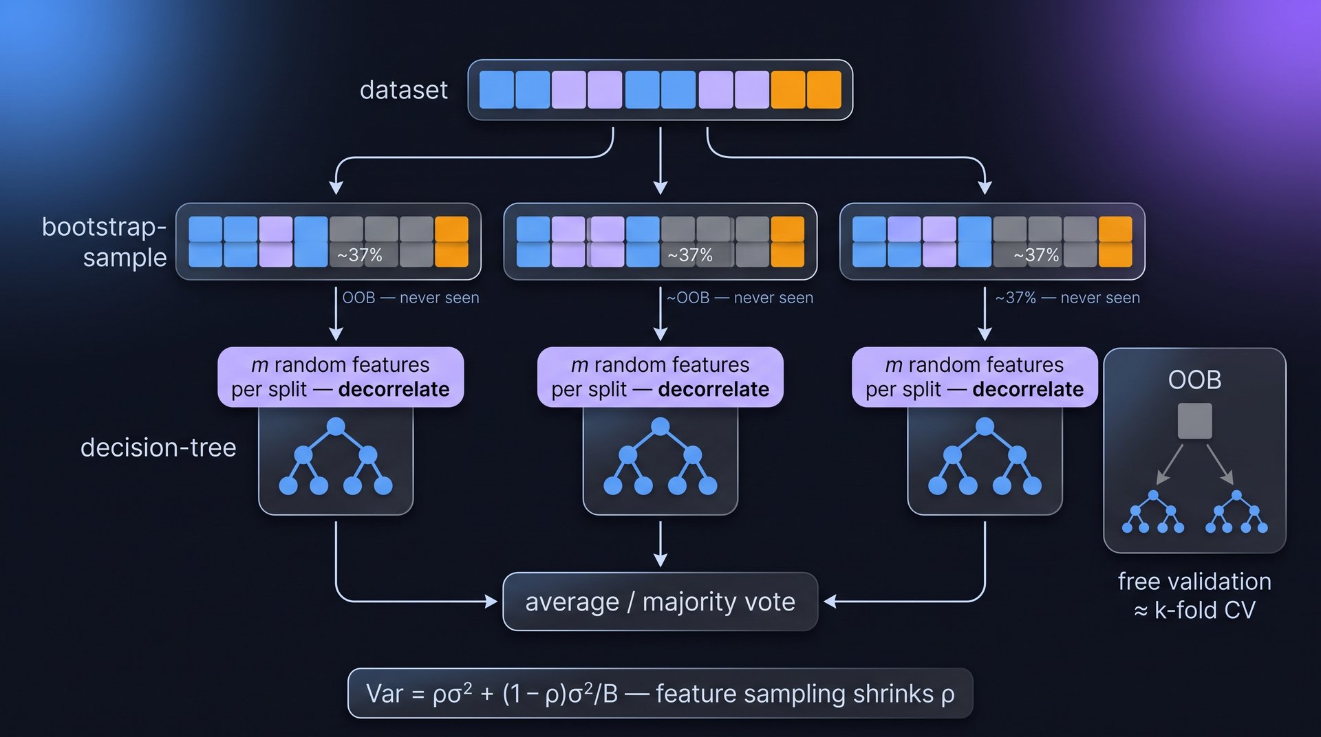
Random forest + OOB error — Unit 8

Input:  N samples, B trees (~500), feature fraction m (√d clf | d/3 reg)
Output: ensemble predictor + free OOB error estimate

1:  for b = 1 … B do
2:      D_b ← bootstrap sample of size N (with replacement)   # ~63% unique
3:      grow a FULL CART tree on D_b, but at EACH split
4:          search only m randomly chosen features            # decorrelation
5:  end for
6:  predict: average (regression) | majority vote (classification)
7:  OOB: score each xᵢ using only the ~37% of trees that never saw it
        # ≈ k-fold CV quality, zero extra cost

Why it works: \(\mathrm{Var}(\text{avg}) = \rho\sigma^2 + \frac{1-\rho}{B}\sigma^2\) — bagging kills the second term, feature subsampling shrinks \(\rho\) and breaks the correlation ceiling.
Pitfall: skipping feature subsampling = plain bagging, stuck at the \(\rho\sigma^2\) floor.

Random forest + OOB — overview figure

Gradient boosting — Unit 8

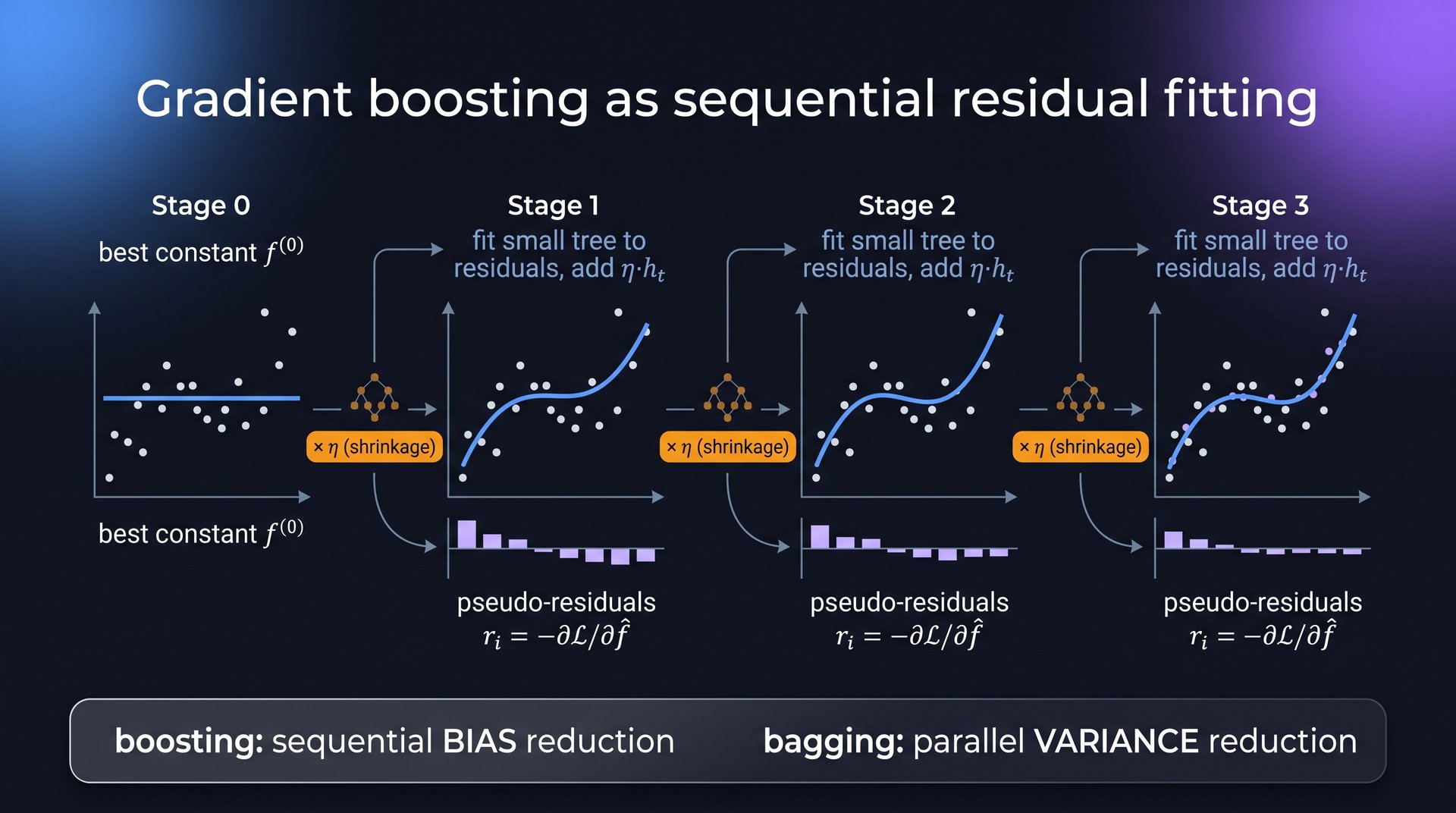
Input:  data, differentiable loss ℒ, shrinkage η (0.01–0.1), rounds T
Output: additive model f̂

1:  f̂⁽⁰⁾ ← argmin_c Σᵢ ℒ(yᵢ, c)                      # best constant
2:  for t = 1 … T do
3:      rᵢ ← − ∂ℒ(yᵢ, f̂⁽ᵗ⁻¹⁾(xᵢ)) / ∂f̂⁽ᵗ⁻¹⁾(xᵢ)      # pseudo-residuals
4:      fit a SMALL tree h_t to {(xᵢ, rᵢ)}             # depth 3–6
5:      f̂⁽ᵗ⁾ ← f̂⁽ᵗ⁻¹⁾ + η · h_t
6:  end for

Why it works: gradient descent in function space — each tree steps against the current loss gradient; sequential bias reduction (bagging reduces variance).
Pitfall: \(\eta\) and \(T\) trade off — tune jointly with early stopping; exponential loss (AdaBoost) is fragile to label noise.

Gradient boosting — overview figure

Permutation importance — Unit 8 / 14

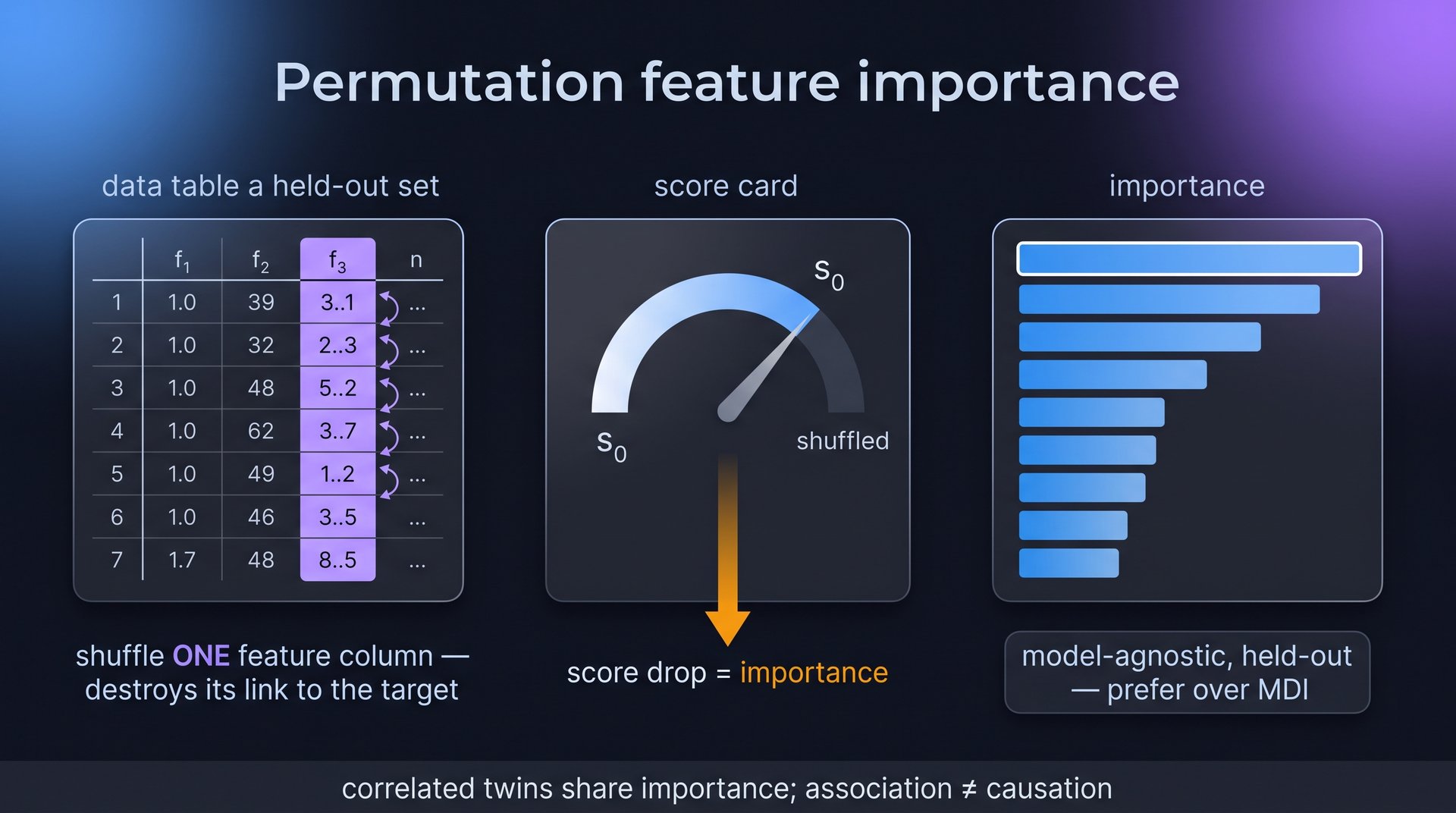
Input:  trained model, HELD-OUT set, score metric S, repeats R
Output: importance per feature

1:  s₀ ← S(model, held-out)                     # baseline
2:  for each feature j:
3:      for r = 1 … R:
4:          shuffle column j across rows (copy of held-out set)
5:          s_{j,r} ← S(model, shuffled set)
6:      importance_j ← s₀ − mean_r s_{j,r}
7:  return features sorted by importance

Why it works: shuffling destroys only the feature–target association; held-out data makes it honest and it is model-agnostic — prefer it over MDI (training-set based, cardinality-biased).
Pitfall: correlated features share importance — the model reads the signal from the twin; association is still not causation.

Permutation importance — overview figure

t-SNE — Unit 9

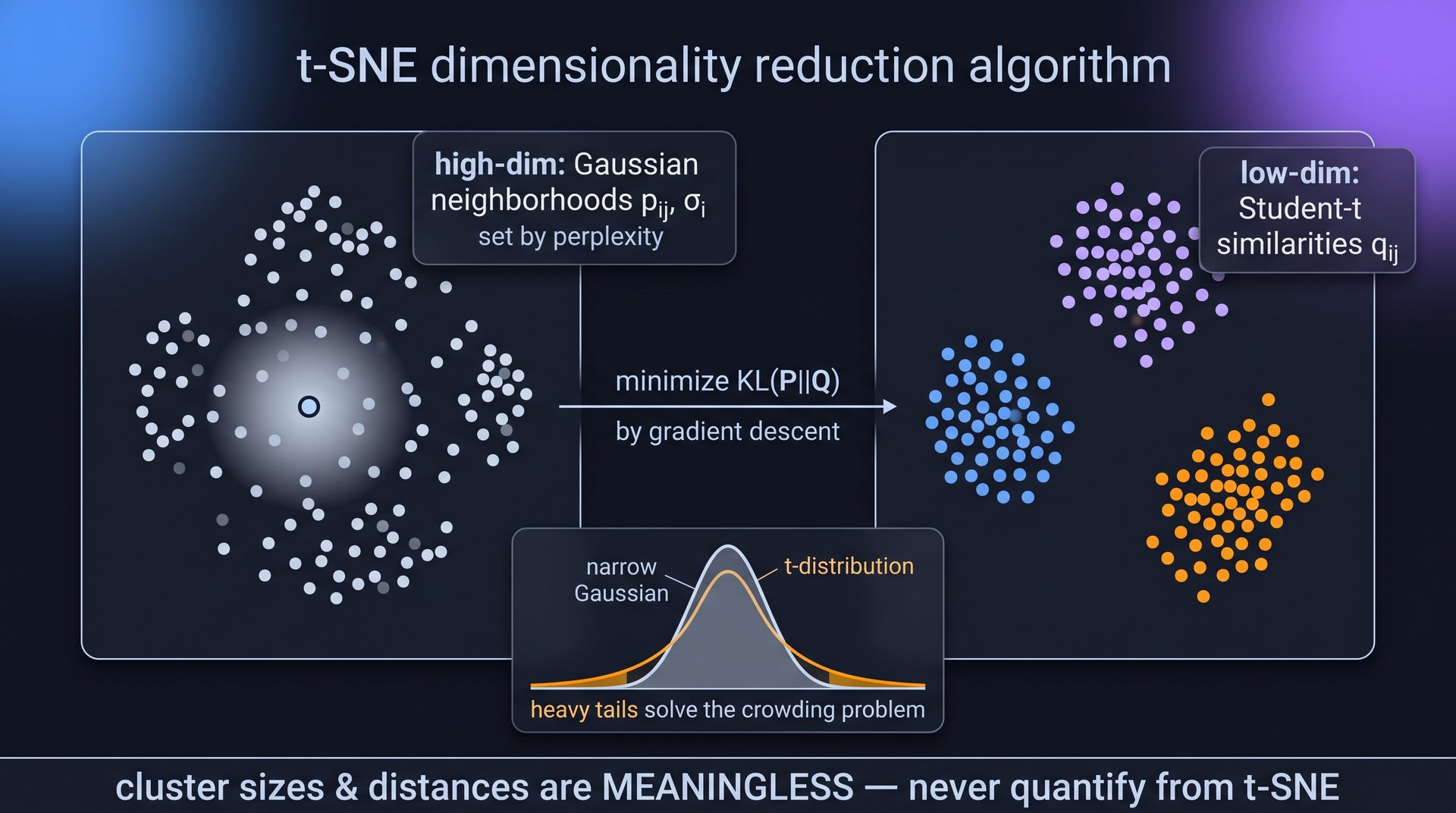
Input:  {xᵢ} high-dim, perplexity (5–50), output dim 2
Output: embedding {yᵢ}

1:  p_{j|i} ← exp(−‖xᵢ−x_j‖²/2σᵢ²) / Σ_{k≠i} exp(−‖xᵢ−x_k‖²/2σᵢ²)
2:  binary-search σᵢ per point so that 2^{H(Pᵢ)} = perplexity
3:  symmetrize:  p_{ij} ← (p_{j|i} + p_{i|j}) / 2N
4:  low-dim similarities (Student-t, heavy tails):
        q_{ij} ← (1+‖yᵢ−y_j‖²)⁻¹ / Σ_{k≠l} (1+‖y_k−y_l‖²)⁻¹
5:  minimize KL(P ‖ Q) over {yᵢ}: gradient descent + momentum, ~1000 iters

Why it works: the heavy-tailed t-distribution solves the crowding problem; the asymmetric KL punishes mapping neighbors far apart → local structure is preserved.
Pitfall: cluster sizes and inter-cluster distances are meaningless; the picture changes with perplexity — never quantify from a t-SNE plot.

t-SNE — overview figure

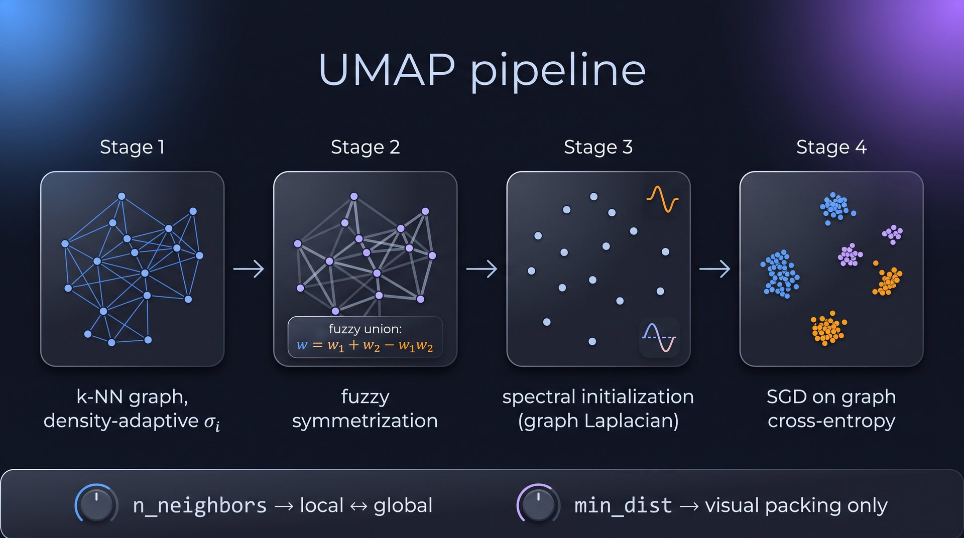
UMAP — Unit 9

Input:  {xᵢ}, n_neighbors, min_dist, output dim 2
Output: embedding {yᵢ}

1:  build k-NN graph (k = n_neighbors); density-adaptive rescaling σᵢ
2:  fuzzy symmetrization:
        w_{ij} ← w_{i→j} + w_{j→i} − w_{i→j} · w_{j→i}
3:  initialize {yᵢ} from SPECTRAL layout (graph-Laplacian eigenvectors)
4:  minimize cross-entropy between high-dim and low-dim edge weights (SGD)

Why it works: the spectral initialization plus graph cross-entropy preserves more global structure than t-SNE and scales to larger N.
Pitfall: same over-reading dangers as t-SNE; n_neighbors sets the local↔︎global trade-off, min_dist only the visual packing.

UMAP — overview figure

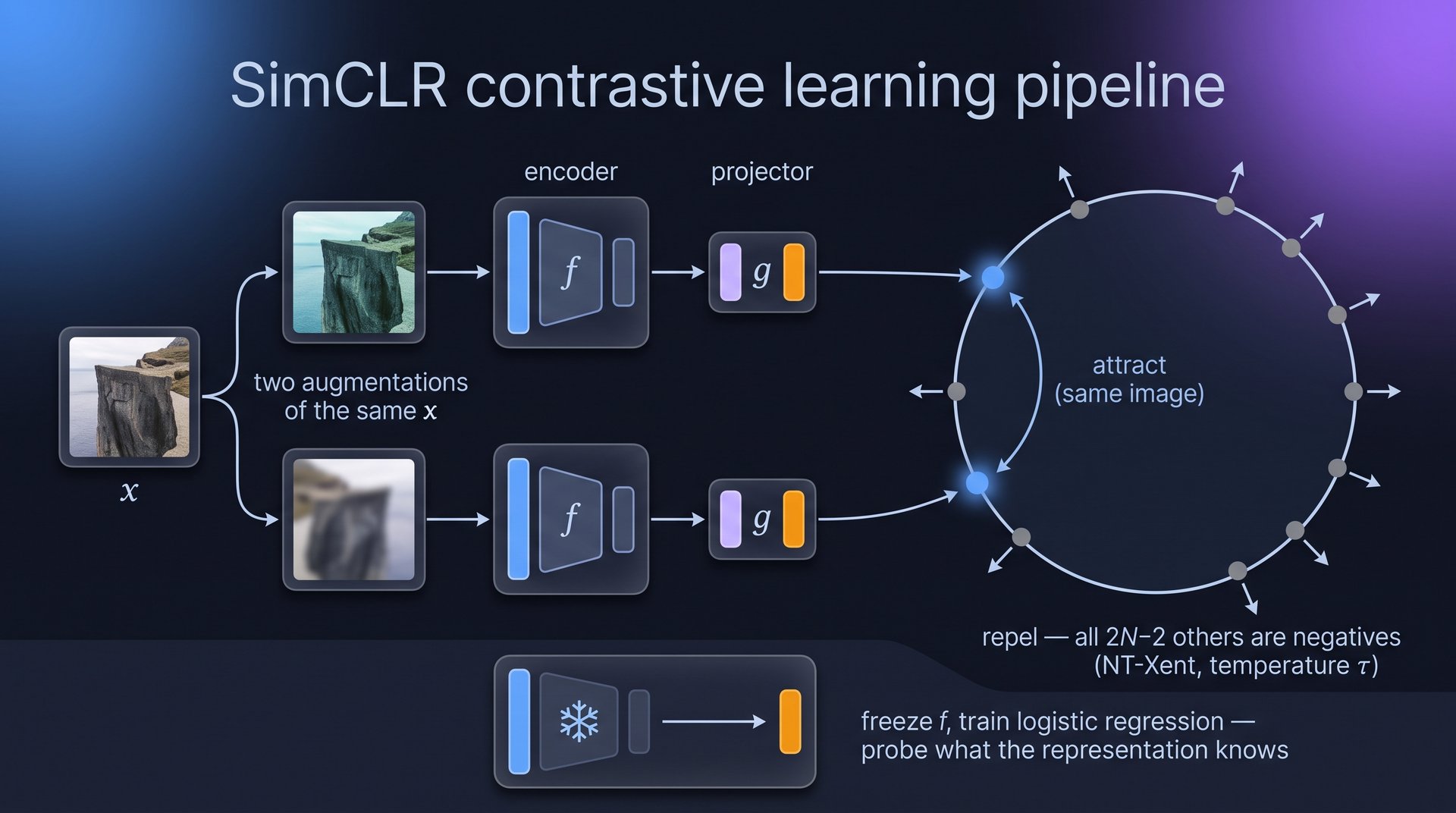
SimCLR + linear probe — Unit 9

Input:  unlabeled batch of N samples, augmentation family 𝒜,
        encoder f, projector g, temperature τ
Output: pretrained encoder f

1:  for each xᵢ: draw two augmentations → 2N views
2:  z_k ← g(f(view_k)); ℓ2-normalize
3:  for each positive pair (i, j):                # two views of same x
4:      ℓ_{i,j} ← −log exp(sim(zᵢ,z_j)/τ) / Σ_{k≠i} exp(sim(zᵢ,z_k)/τ)
        # sim = cosine; all other 2N−2 samples act as negatives (NT-Xent)
5:  loss ← mean over positive pairs; update f, g

Evaluate — linear probe: freeze f; train logistic regression on {f(xᵢ), yᵢ};
    test accuracy measures what the representation already knows.

Why it works: pulls augmented views together and pushes everything else apart — the invariances are defined by the augmentation family.
Pitfall: augmentations encode what should NOT matter; choose them from domain knowledge (don’t flip if chirality matters).

SimCLR + linear probe — overview figure

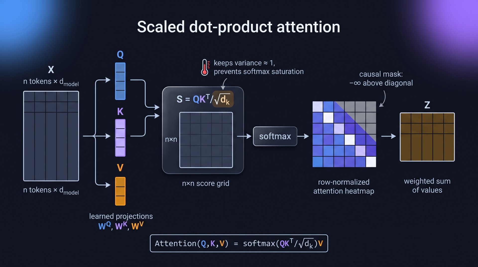
Scaled dot-product attention — Unit 10

Input:  token embeddings X ∈ ℝ^{n×d_model}; learned W^Q, W^K, W^V
Output: contextualized tokens Z

1:  Q ← X W^Q;   K ← X W^K;   V ← X W^V
2:  S ← Q Kᵀ / √d_k                        # scores, n×n
3:  causal mask (decoders): S_{ij} ← −∞ for j > i    # no peeking ahead
4:  A ← softmax(S, row-wise)               # each row sums to 1
5:  Z ← A V                                # weighted sum of values

Boxed:  Attention(Q, K, V) = softmax(QKᵀ/√d_k) V
Cross-attention: Q from sequence A; K, V from sequence B

Why it works: \(\sqrt{d_k}\) keeps score variance \(\approx 1\), preventing softmax saturation; \(-\infty\) before softmax = exactly zero weight.
Pitfall: \(O(n^2)\) memory in sequence length; forgetting the scale factor stalls training.

Scaled dot-product attention — overview figure

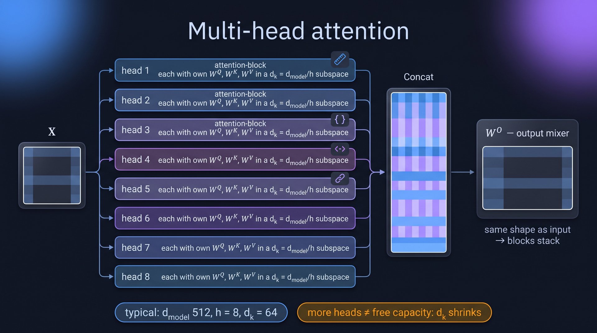
Multi-head attention — Unit 10

Input:  X ∈ ℝ^{n×d_model}, heads h, per-head d_k = d_v = d_model/h
Output: MultiHead(X) ∈ ℝ^{n×d_model}       # same shape as input

1:  for i = 1 … h  (in parallel):
2:      head_i ← Attention(X W_i^Q, X W_i^K, X W_i^V)
3:  C ← Concat(head_1, …, head_h)           # n × (h·d_v)
4:  return C W^O                            # output mixer restores d_model

Typical: d_model = 512, h = 8, d_k = 64

Why it works: heads attend in independent learned subspaces and specialize (position, syntax, …); shape-in = shape-out makes blocks stackable.
Pitfall: more heads means smaller \(d_k\) per head at fixed \(d_{model}\) — not free capacity.

Multi-head attention — overview figure

Transformer block (+ positional encoding) — Unit 10

Input:  X ∈ ℝ^{n×d_model}
Output: same shape — stack L identical blocks (L = 6 … 96)

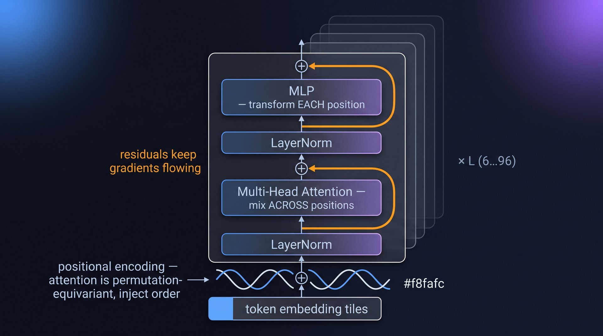
Before block 1 (attention is permutation-equivariant — inject order):
    PE(pos, 2i)   = sin(pos / 10000^{2i/d_model})
    PE(pos, 2i+1) = cos(pos / 10000^{2i/d_model})
    X ← token embeddings + PE

One block (pre-norm):
1:  X ← X + MultiHead(LayerNorm(X))          # mix across positions + residual
2:  X ← X + MLP(LayerNorm(X))                # per-position 2-layer FF + residual

Why it works: attention mixes across positions, the MLP transforms each position; residual connections keep gradients flowing through deep stacks.
Pitfall: dropping positional encodings — the model literally cannot see token order.

Transformer block — overview figure

Vision Transformer forward pass — Unit 10

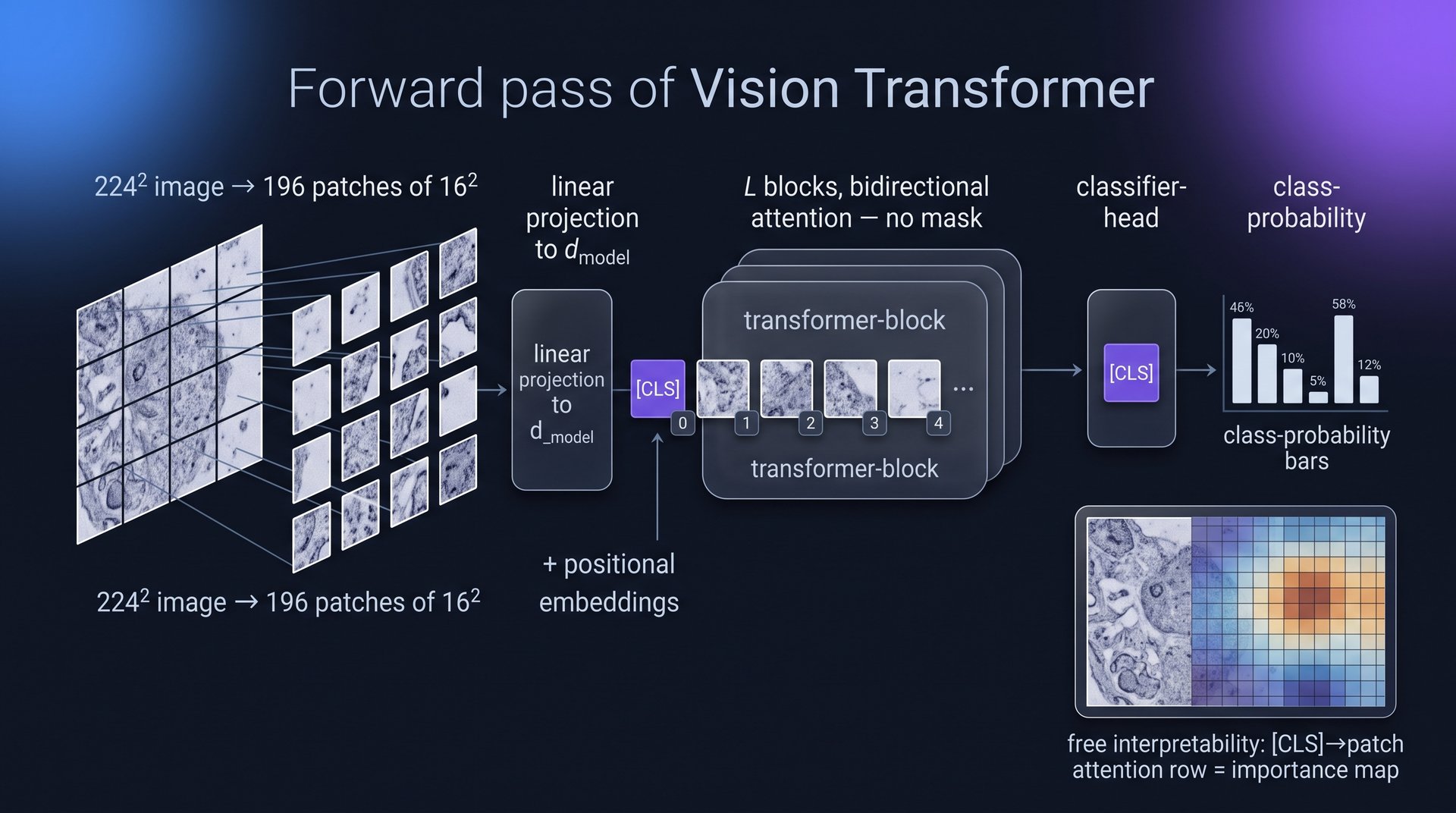
Input:  image 224×224, patch size 16, transformer of L blocks
Output: class prediction

1:  split image into (224/16)² = 196 patches;  flatten each
2:  linear-project each patch to d_model;  prepend learned [CLS] token
3:  add positional embeddings
4:  run L transformer blocks (bidirectional attention, no mask)
5:  ŷ ← classifier head on the final [CLS] representation

Free interpretability: the softmax row [CLS → patches], reshaped to the
14×14 grid, is a patch-importance heatmap — one forward pass, no extra cost.

Why it works: treats the image as a token sequence — no convolutional inductive bias, traded for large-scale pretraining.
Pitfall: on small datasets CNNs win — ViT needs pretraining to recover what locality priors gave for free.

Vision Transformer — overview figure

VAE training step — Unit 11

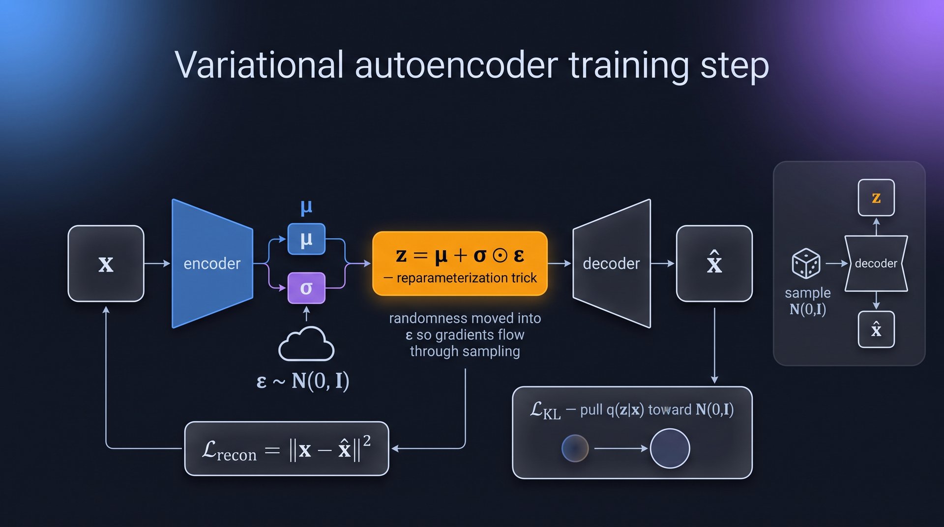
Input:  batch x; encoder → (μ_φ(x), σ_φ(x)); decoder g_θ; prior N(0, I)
Output: trained θ, φ;  generation: z ~ N(0,I) → g_θ(z)

1:  ε ← sample N(0, I)
2:  z ← μ_φ(x) + σ_φ(x) ⊙ ε                 # reparameterization trick
3:  x̂ ← g_θ(z)
4:  L_recon ← ‖x − x̂‖²
5:  L_KL ← ½ Σ_j ( μ_j² + σ_j² − log σ_j² − 1 )     # closed form (Gaussians)
6:  L ← L_recon + β · L_KL;   gradient step on θ, φ

Why it works: minimizing \(L\) maximizes the ELBO; reparameterization moves the randomness into \(\epsilon\) so gradients flow through the sampling step.
Pitfall: posterior collapse (encoder ignores \(x\)) — warm \(\beta\) up from 0; \(\beta>1\) disentangles but blurs.

VAE — overview figure

DDPM training — Unit 11

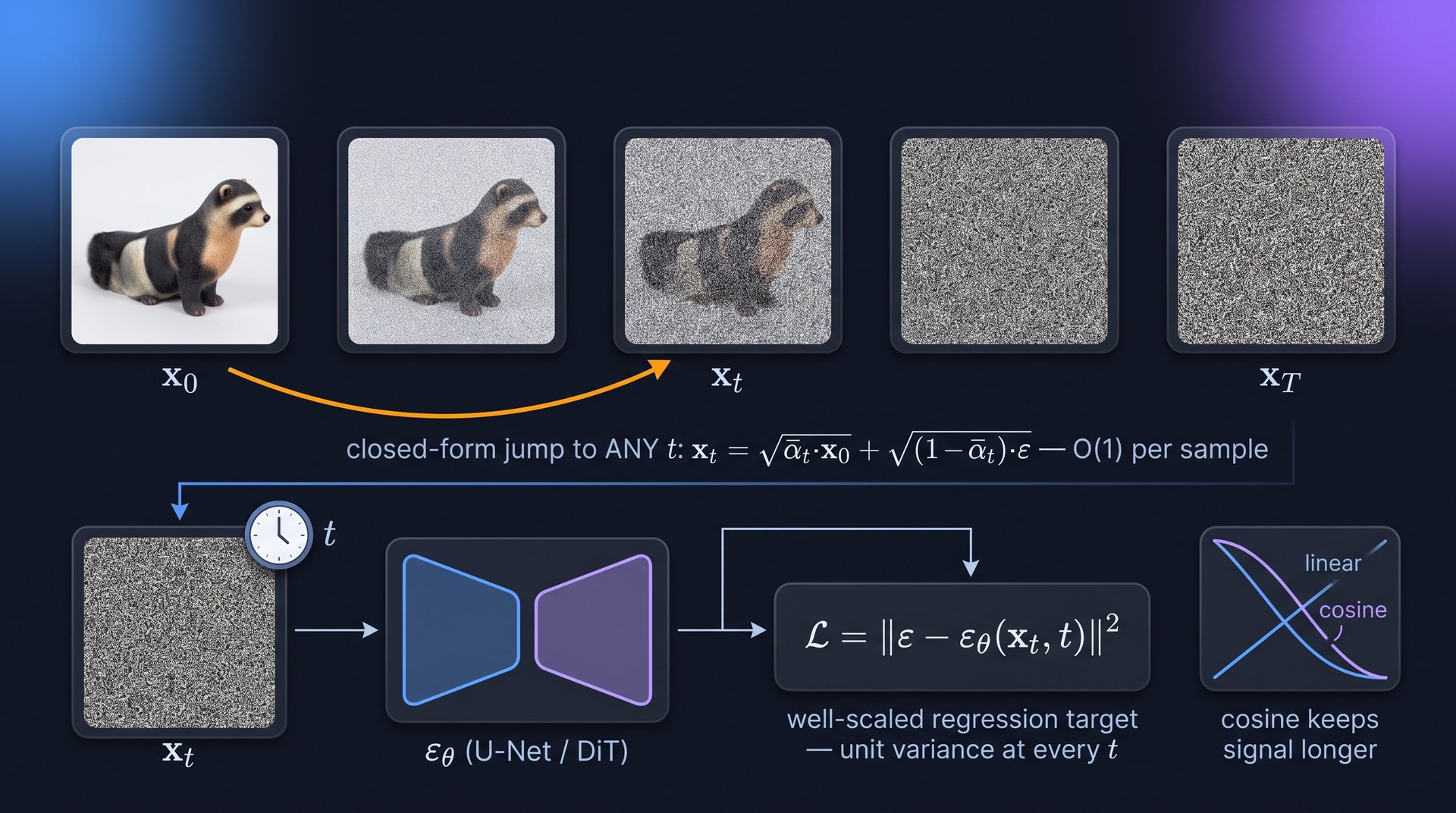
Input:  data x₀, steps T (~1000), schedule β₁…β_T, ᾱ_t = Π_{s≤t}(1−β_s),
        denoiser ε_θ (U-Net or DiT)
Output: trained ε_θ

1:  repeat
2:      x₀ ~ data;   t ~ Uniform{1…T};   ε ~ N(0, I)
3:      x_t ← √ᾱ_t · x₀ + √(1−ᾱ_t) · ε        # closed-form jump to ANY t
4:      L ← ‖ ε − ε_θ(x_t, t) ‖²
5:      gradient step on θ
6:  until converged

Why it works: predicting \(\epsilon\) is a well-scaled regression target (unit variance at every \(t\)) — one network serves all noise levels; the closed-form jump makes training \(O(1)\) per sample, not \(O(T)\).
Pitfall: the noise schedule matters — cosine keeps signal longer than linear and spends capacity where learning is informative.

DDPM training — overview figure

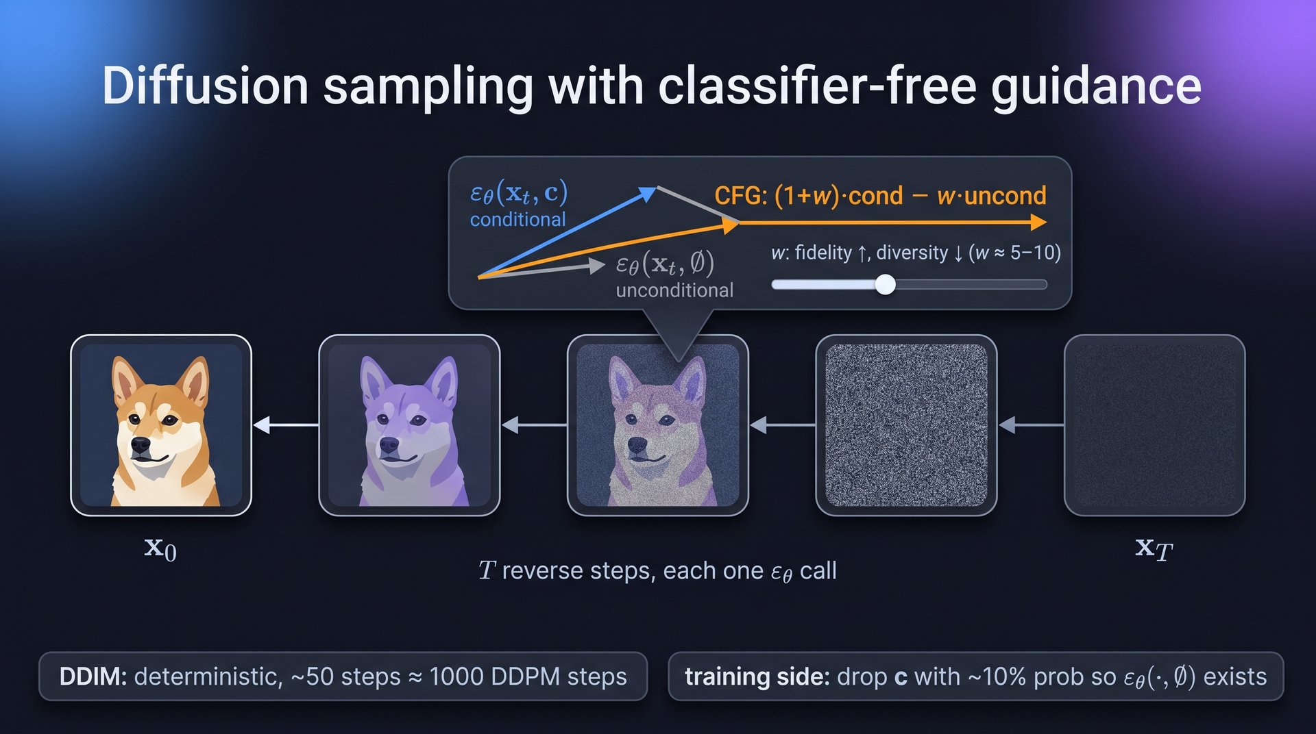
Diffusion sampling + classifier-free guidance — Unit 11

Input:  trained ε_θ, guidance scale w, condition c
Output: sample x₀

1:  x_T ← N(0, I)
2:  for t = T … 1 do
3:      ε̂ ← (1+w) · ε_θ(x_t, c)  −  w · ε_θ(x_t, ∅)   # CFG
4:      μ_t, σ_t ← posterior formulas from ε̂
5:      x_{t−1} ← μ_t + σ_t · z,   z ~ N(0,I)   (z = 0 at t = 1)
6:  end for
7:  return x₀

DDIM: same trained ε_θ, deterministic steps → ~50 steps ≈ 1000 DDPM steps
CFG training side: drop condition c with ~10% probability so ε_θ(·,∅) exists

Why it works: runs the learned reverse process from pure noise; \(w\) amplifies the conditional direction relative to unconditional.
Pitfall: larger \(w\) = higher fidelity, lower diversity (typical \(w \approx 5\)–10); DDPM sampling costs \(T\) network calls.

Diffusion sampling + CFG — overview figure

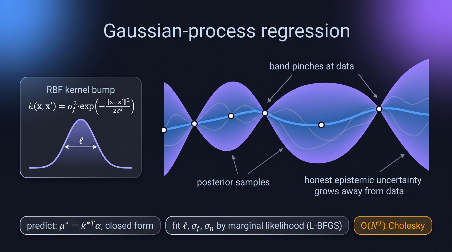
GP regression — Unit 12

Input:  data (X, y); kernel k, e.g. RBF k(x,x′) = σ_f² exp(−‖x−x′‖²/2ℓ²);
        noise σ_n²
Output: predictive mean and variance at x*

1:  K ← [k(xᵢ,x_j)] ∈ ℝ^{N×N};    k* ← [k(x*, xᵢ)]
2:  L ← cholesky(K + σ_n² I)                    # O(N³), once
3:  α ← Lᵀ \ (L \ y)
4:  μ*(x*)  ← k*ᵀ α                              # posterior mean
5:  σ*²(x*) ← k(x*,x*) − k*ᵀ (K + σ_n² I)⁻¹ k*   # posterior variance

Hyperparameters (ℓ, σ_f, σ_n): maximize the marginal likelihood
  log p(y|X) = −½ yᵀ(K+σ_n²I)⁻¹y − ½ log|K+σ_n²I| − (N/2) log 2π   (L-BFGS)

Why it works: conditioning a joint Gaussian on observations is closed-form; variance grows away from data — honest epistemic uncertainty. (Both formulas: write from memory.)
Pitfall: \(O(N^3)\) scaling; the marginal likelihood is multimodal — restart the optimizer.

GP regression — overview figure

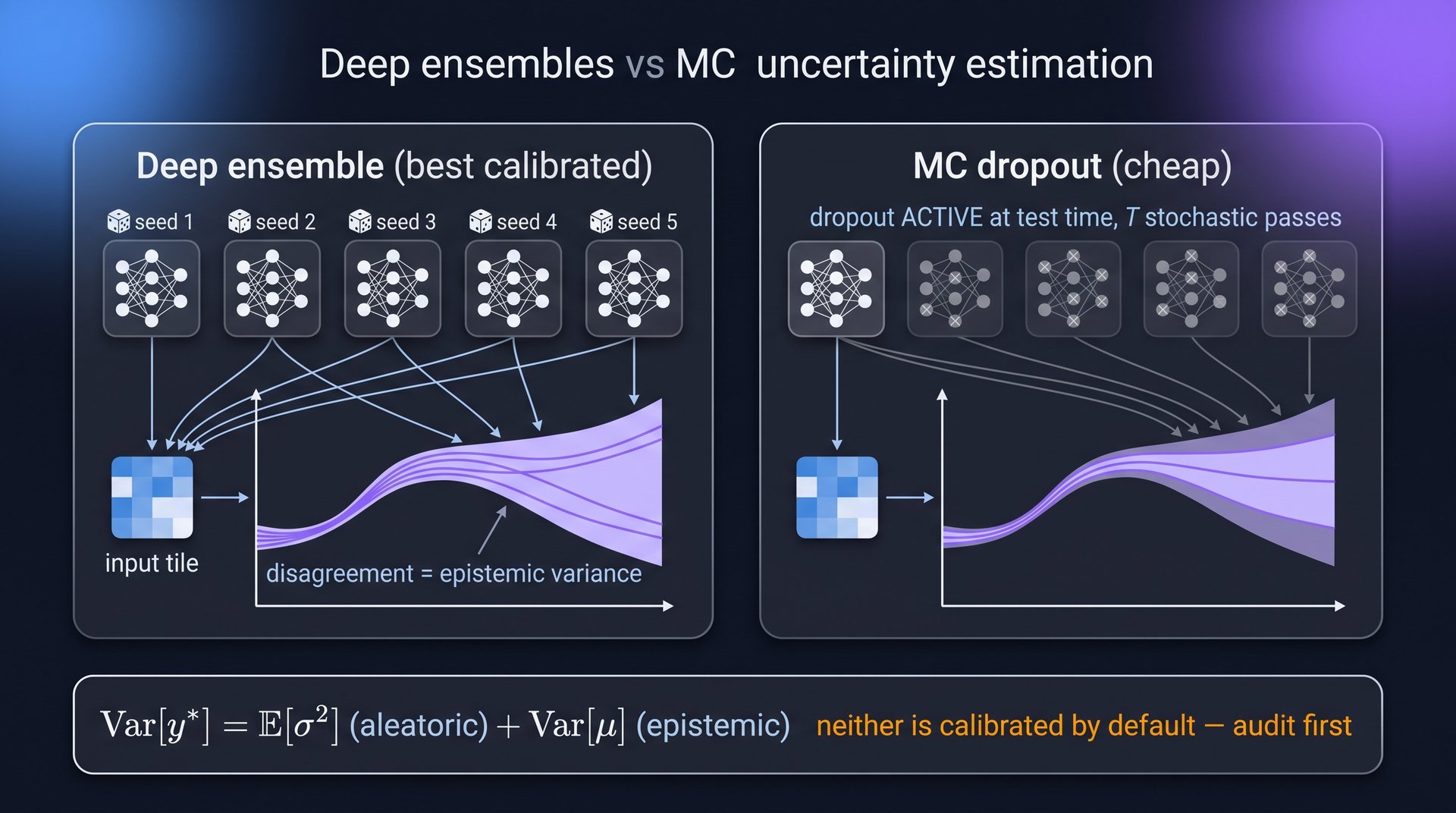
Uncertainty by sampling: ensembles & MC dropout — Unit 12

Deep ensemble (best calibrated):
1:  train M (~5) networks — same architecture, different random seeds
2:  collect predictions ŷ_1 … ŷ_M
3:  mean  ȳ ← (1/M) Σ_m ŷ_m
4:  epistemic variance ← (1/M) Σ_m (ŷ_m − ȳ)²

MC dropout (cheap approximation):
1:  keep dropout ACTIVE at test time
2:  run T stochastic forward passes on the same input
3:  prediction ← mean;   uncertainty ← variance across passes

Why it works: both sample “plausible models” — their disagreement is the epistemic term in \(\mathrm{Var}[y^*] = \underbrace{\mathbb{E}[\sigma^2]}_{\text{aleatory}} + \underbrace{\mathrm{Var}[\mu]}_{\text{epistemic}}\).
Pitfall: neither is calibrated by default — audit before trusting the bands (next slide).

Ensembles & MC dropout — overview figure

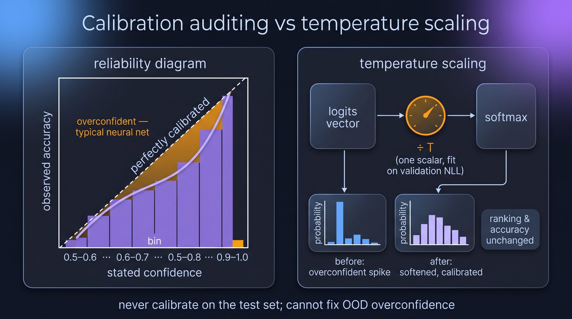
Calibration audit + temperature scaling — Unit 12

Audit (reliability diagram), on a HELD-OUT set:
1:  bin predictions by stated confidence (0.5–0.6, …, 0.9–1.0)
2:  per bin: observed accuracy  vs  mean stated confidence
3:  plot; on the diagonal = calibrated, below = overconfident (typical NN)

Temperature scaling (post-hoc fix):
1:  learn ONE scalar T minimizing NLL of softmax(logits / T) on validation
2:  deploy softmax(logits / T)      # ranking/accuracy unchanged
Alternatives: Platt scaling, isotonic regression

Why it works: one scalar fixes systematic overconfidence without touching the model or its accuracy.
Pitfall: calibrating on the test set; recalibration cannot fix overconfidence far off the training manifold (OOD).

Calibration + temperature scaling — overview figure

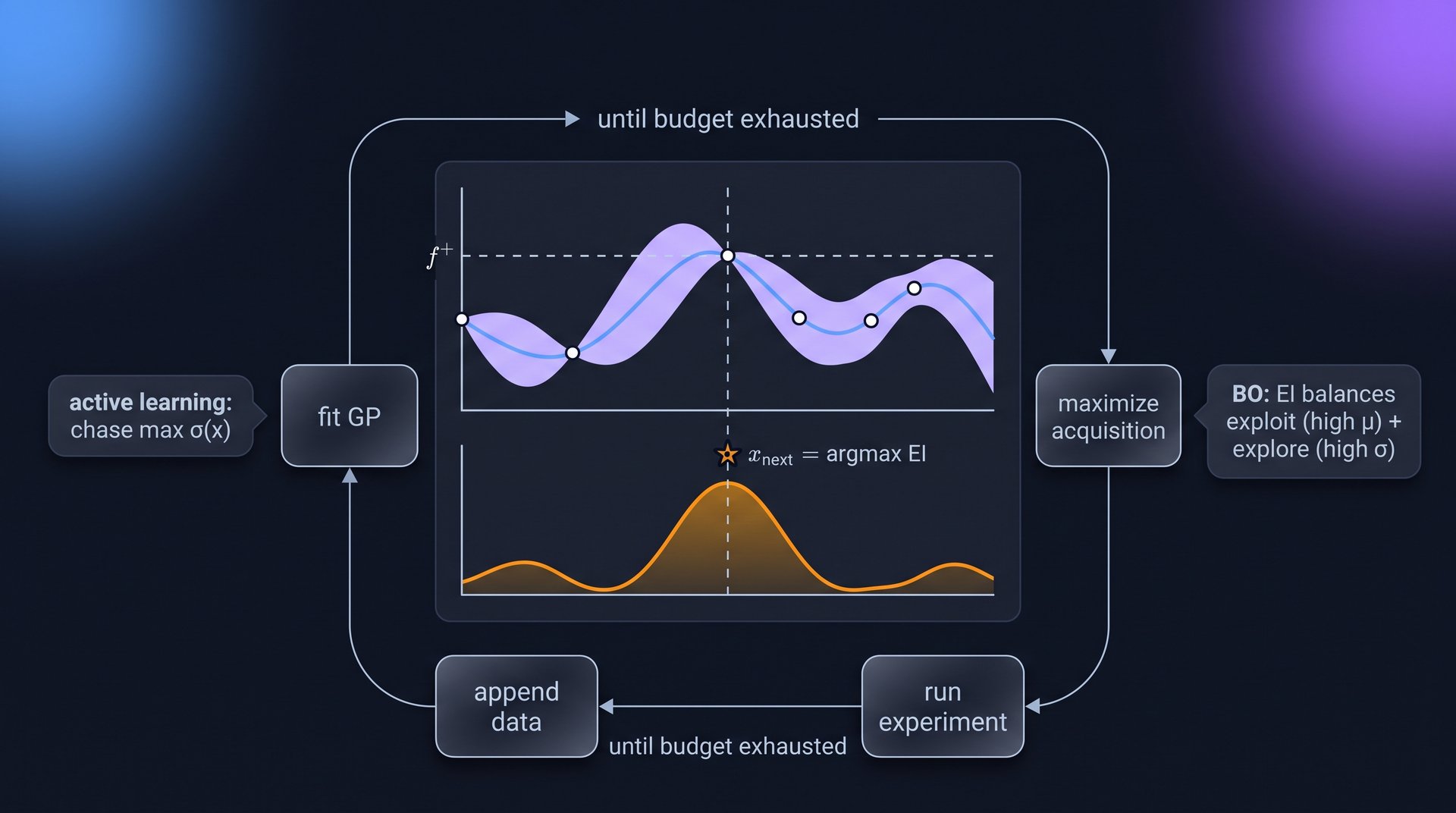
Active learning & Bayesian optimization — Unit 12

Input:  small initial dataset, GP surrogate, experiment budget
Output: mapped function / located optimum in few experiments

1:  repeat until budget exhausted:
2:      fit GP on current data (hyperparams by marginal likelihood)
3:      choose next point:
          active learning:        x_next ← argmax_x σ*(x)     # max epistemic
          Bayesian optimization:  x_next ← argmax_x EI(x)
            EI(x) = (μ(x) − f⁺ − ε)·Φ(Z) + σ(x)·φ(Z),
            Z = (μ(x) − f⁺ − ε)/σ(x),  f⁺ = best observed value
4:      run the experiment at x_next;  append (x_next, y) to data
5:  end

Why it works: EI’s two terms balance exploitation (high mean) and exploration (high variance) — the GP’s honest uncertainty drives the search.
Pitfall: pure variance-chasing maps the function but never optimizes it; the \(\epsilon\) knob shifts the explore/exploit balance.

Active learning & BO — overview figure

PINN training loop — Unit 13

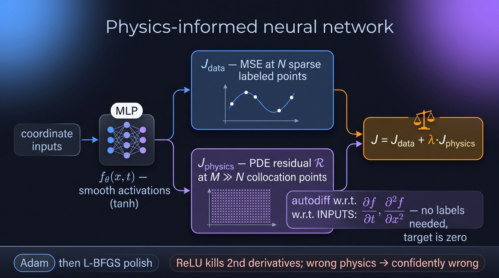
Input:  sparse data {(xᵢ, yᵢ)}ᴺ, PDE residual ℛ, collocation points {x_j}ᴹ
        (M ≫ N, unlabeled), weight λ, MLP f_θ with SMOOTH activations (tanh)
Output: trained field f_θ

1:  repeat
2:      J_data ← (1/N) Σᵢ ‖yᵢ − f_θ(xᵢ)‖²
3:      autodiff w.r.t. INPUTS at collocation points: ∂f_θ/∂t, ∂²f_θ/∂x², …
4:      J_physics ← (1/M) Σ_j ‖ℛ(f_θ, x_j)‖²        # target is zero: NO labels
5:      J ← J_data + λ · J_physics
6:      gradient step on θ                            # Adam, then L-BFGS polish
7:  until converged

Why it works: the physics residual supervises everywhere data is missing — MAP estimation with a physics prior.
Pitfall: ReLU’s zero second derivative kills the residual; gradient imbalance between the two terms (adaptive \(\lambda\)); wrong physics → confidently wrong solution.

PINN training loop — overview figure

Lagaris substitution — Unit 13

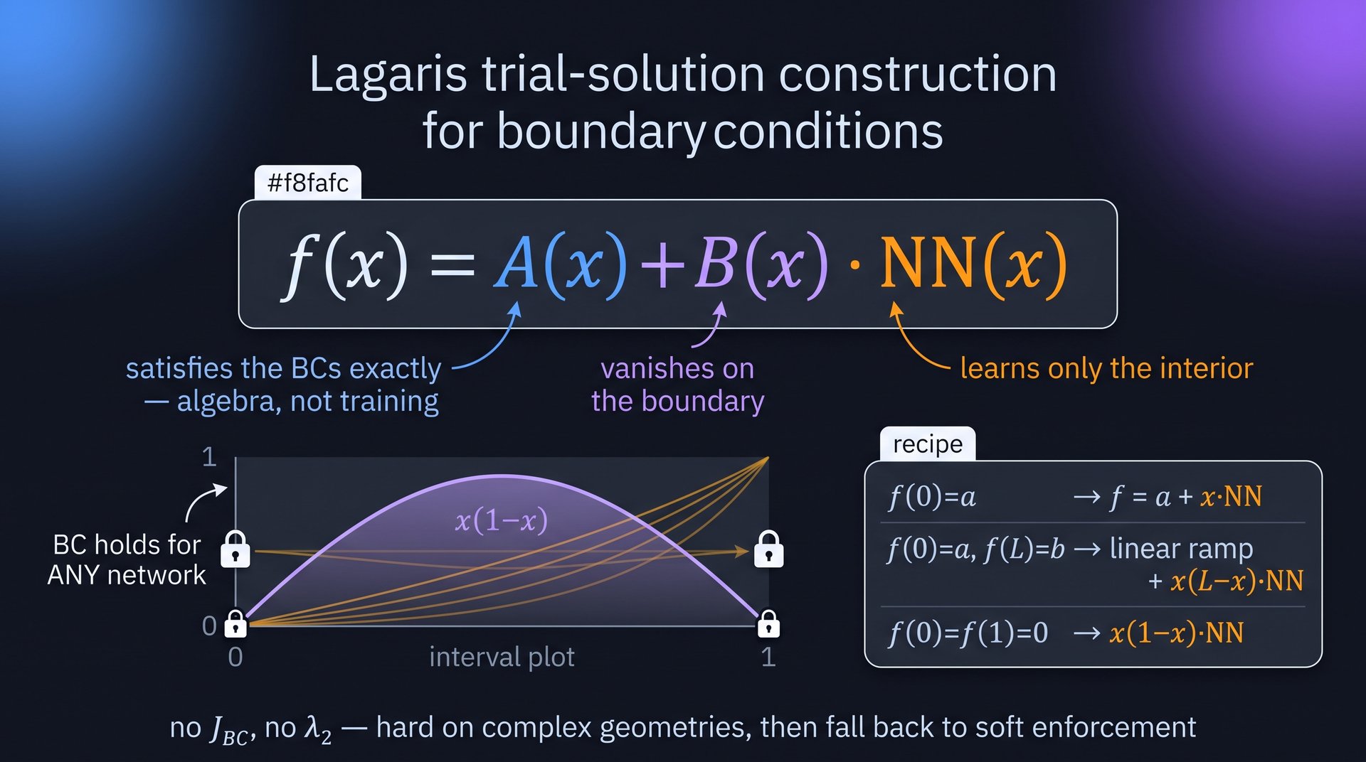
Goal:   solve an ODE/PDE with boundary conditions satisfied EXACTLY
Input:  equation with residual ℛ, boundary/initial conditions

1:  choose A(x) that satisfies all BCs            # by hand — algebra, not training
2:  choose B(x) that vanishes on the boundary
3:  trial solution   f(x) = A(x) + B(x) · NN(x)   # BCs hold for ANY network
4:  train the NN by minimizing Σ_j ℛ(f, x_j)² at collocation points

Recipes:
  f(0) = a            →  f = a + x · NN(x)
  f(0) = a, f(L) = b  →  f = a + (x/L)(b−a) + x(L−x) · NN(x)
  f(0) = f(1) = 0     →  f = x(1−x) · NN(x)

Why it works: the boundary term is exact before training starts — no \(J_{BC}\), no \(\lambda_2\); the NN learns only the unknown interior deviation.
Pitfall: constructing \(A, B\) is easy on intervals and boxes, genuinely hard on complex geometries — then fall back to soft enforcement.

Lagaris substitution — overview figure

Perturbation sensitivity analysis — Unit 14

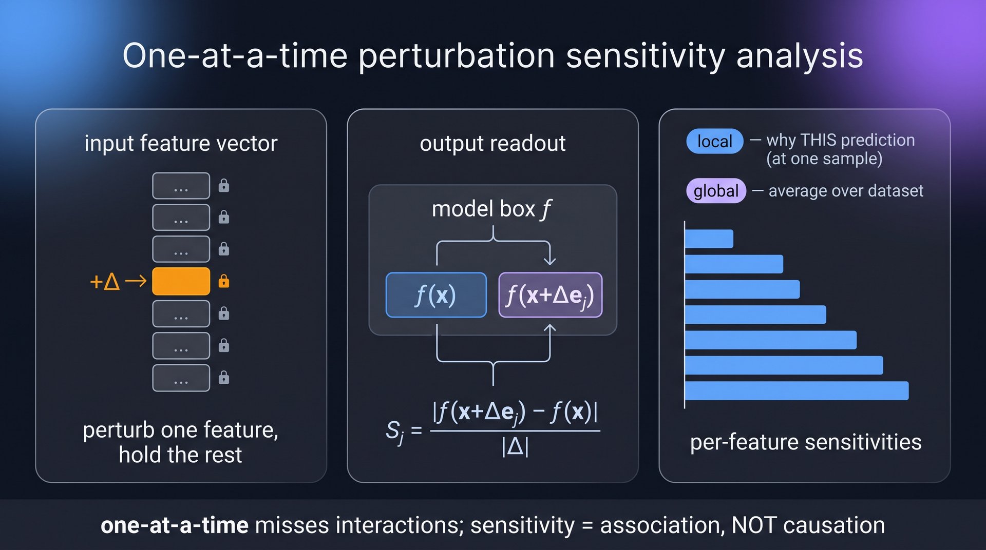
Input:  trained model f, input x, perturbation size Δ
Output: per-feature sensitivity S_j

1:  for each feature j:
2:      S_j ← | f(x + Δ·e_j) − f(x) | / |Δ|      # one-at-a-time
3:  local explanation:  report S_j at the sample of interest
        ("why THIS prediction")
4:  global importance:  average S_j over the dataset
        ("which features matter on average")

Why it works: the model-agnostic first look at feature relevance; complements SHAP (axiomatic attribution) and permutation importance (held-out, association-destroying).
Pitfall: one-at-a-time misses interactions; sensitivity is association, not causation — no attribution method crosses that gap without domain knowledge.

Perturbation sensitivity — overview figure

Continue

← Back: Unit 14 — Explainability, Limits, and Scientific Trust
All courses

Mathematical Foundations of AI & MLAppendix: Algorithm Compendium

How to use this deck

Data splitting & k-fold cross-validation — Unit 1

Data splitting & k-fold CV — overview figure

Ordinary least squares (+ ridge) — Unit 2

OLS + ridge — overview figure

PCA via SVD — Unit 2

PCA via SVD — overview figure

Gradient descent, SGD, minibatch — Unit 3

GD / SGD / minibatch — overview figure

Newton’s method — Unit 3

Newton’s method — overview figure

Logistic regression training — Unit 3

Logistic regression — overview figure

MLP forward pass — Unit 4

MLP forward pass — overview figure

Backpropagation — Unit 4

Backpropagation — overview figure

2D convolution (multi-channel) — Unit 4

2D convolution — overview figure

k-means (Lloyd + k-means++) — Unit 5

k-means — overview figure

EM for Gaussian mixtures — Unit 5

EM for GMM — overview figure

Autoencoder training + anomaly detection — Unit 5

Autoencoder — overview figure

Momentum & Nesterov — Unit 6

Momentum & Nesterov — overview figure

AdaGrad + training stabilizers — Unit 6

AdaGrad + stabilizers — overview figure

MLE and MAP estimation — Unit 7

MLE & MAP — overview figure

CART: growing a decision tree — Unit 8

CART — overview figure

Random forest + OOB error — Unit 8

Random forest + OOB — overview figure

Gradient boosting — Unit 8

Gradient boosting — overview figure

Permutation importance — Unit 8 / 14

Permutation importance — overview figure

t-SNE — Unit 9

t-SNE — overview figure

UMAP — Unit 9

UMAP — overview figure

SimCLR + linear probe — Unit 9

SimCLR + linear probe — overview figure

Scaled dot-product attention — Unit 10

Scaled dot-product attention — overview figure

Multi-head attention — Unit 10

Multi-head attention — overview figure

Transformer block (+ positional encoding) — Unit 10

Transformer block — overview figure

Vision Transformer forward pass — Unit 10

Vision Transformer — overview figure

VAE training step — Unit 11

VAE — overview figure

DDPM training — Unit 11

DDPM training — overview figure

Diffusion sampling + classifier-free guidance — Unit 11

Diffusion sampling + CFG — overview figure

GP regression — Unit 12

GP regression — overview figure

Uncertainty by sampling: ensembles & MC dropout — Unit 12

Ensembles & MC dropout — overview figure

Calibration audit + temperature scaling — Unit 12

Calibration + temperature scaling — overview figure

Active learning & Bayesian optimization — Unit 12

Active learning & BO — overview figure

PINN training loop — Unit 13

PINN training loop — overview figure

Lagaris substitution — Unit 13

Lagaris substitution — overview figure

Perturbation sensitivity analysis — Unit 14

Perturbation sensitivity — overview figure

Continue

Mathematical Foundations of AI & ML
Appendix: Algorithm Compendium