Machine Learning for Characterization and Processing
Unit 11: Physics-constrained ML patterns for the lab

AI 4 Materials / KI-Materialtechnologie

Prof. Dr. Philipp Pelz

FAU Erlangen-Nürnberg

§A · From MFML theory to lab patterns

01. The MFML W13 toolkit (we will not re-derive these)

Tool	One-line summary	When to reach for it
PINN loss decomposition	\(J = J_{\text{data}} + \lambda J_{\text{phys}} + \lambda_b J_{\text{BC}}\)	PDE residual is known and cheap to evaluate
Automatic differentiation	Exact \(\partial f_\theta / \partial x\) inside the loss	Needed for any PDE/ODE residual term
Soft constraint	Penalty in the loss	Easy to add; constraint only approximate
Hard constraint	Built into the architecture (Lagaris)	Constraint must be exact, e.g. BCs, mass
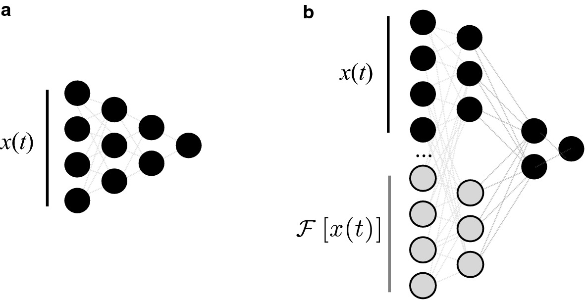
DeepONet / FNO	Learn an operator \(u \mapsto G(u)\)	Many similar PDE instances, fast inference
HNN / equivariant nets	Symmetries / conservation by construction	Energy, momentum, point-group symmetry
SINDy	Sparse regression on a derivative dictionary	Discover the governing equation itself

Note

The math lives in MFML W13 — which this term lands after this unit (Mon 13.07), so treat this table as a preview, not a recap. Today we ask: which of these do I pick up in the lab, and what breaks?

02. Why constrained ML in labs

• A pure-data CNN on grain-size histograms predicts negative grain sizes at the tail of the test set.

• A neural MD surrogate trained only on energies drifts; total energy in a long roll-out decays by 8% per ns.

• A melt-pool surrogate fits training pyrometer traces beautifully but its predicted heat flux can be negative — implying spontaneous heat flow against the gradient.

Warning

Each is a real failure mode. Constraints exist to make these impossible by construction, not to be patched after the fact.

03. What physics to enforce in materials labs

A working checklist for any new ML model in our group:

• Thermodynamic admissibility: \(\Delta G \le 0\) for spontaneous transitions; entropy non-decreasing.
• Kinematic constraints: positive stiffness (\(d\sigma/d\epsilon > 0\) in elastic regime), monotonic loading, \(f_k \ge 0\) for fractions.

• Conservation: mass balance in / out, charge neutrality, sum of phase fractions \(=1\).
• Symmetry: crystal point group on tensors, isotropy of an amorphous sample, periodicity of a unit cell.

• Units & dimensions: every output term must be dimensionally homogeneous with the equation it enters.

Note

For every line of this checklist, decide before training whether a violation should be impossible (hard), penalized (soft), or merely monitored.

§B · Pattern A — Soft-constrained CNN for diffraction inversion

04. Setup: phase-fraction inference from XRD

• Input: 1D XRD pattern, intensity vs \(2\theta\), length ~4000 bins.
• Output: phase fractions \(f_k\) for \(k = 1, \dots, K\) phases.
• Hard requirements: \[f_k \ge 0, \qquad \sum_{k=1}^{K} f_k = 1.\]
• Backbone: 1D U-Net or ResNet-1D with a softmax head.

• Forward operator (Rietveld) is well known: phase mix \(\to\) pattern.
• Inverse operator is the part we need to learn — and the part where the network can hallucinate.

Note

The forward direction is known physics; only the ill-posed inverse is learned — and that is exactly where hallucination lives.

05. The constraint — softmax is not enough

• A softmax head guarantees \(\sum_k f_k = 1\) and \(f_k \ge 0\) — but says nothing about which phases are physically reachable.

• Let \(\mathcal{L}\) be the known phase library for the alloy system being measured. Add a soft regularizer that punishes mass on phases outside the library: \[ \mathcal{L}_{\text{phys}} = \lambda \sum_{k \notin \mathcal{L}} f_k^2 \]

• Total loss: \[ J = J_{\text{data}} + \lambda \sum_{k \notin \mathcal{L}} f_k^2. \]

Note

Softmax buys the simplex constraint for free; the phase library still has to be added as an explicit penalty.

06. What goes wrong without it

• Sample: Fe–Cu binary, ~30 wt% Cu.
• Library \(\mathcal{L} = \{\alpha\text{-Fe}, \gamma\text{-Fe}, \text{fcc-Cu}\}\).
• Unconstrained CNN, trained on a noisy dataset, returns:
  • 0.41 \(\alpha\)-Fe
  • 0.22 \(\gamma\)-Fe
  • 0.19 fcc-Cu
  • 0.18 FeAl\(_3\) — a phase that cannot exist in an Fe–Cu sample.

The network is using a phase that visually fits a peak it cannot otherwise explain. Adding \(\mathcal{L}_{\text{phys}}\) forces it to attribute that intensity to a peak overlap or to the noise model instead.

Warning

An unconstrained network will happily invent a thermodynamically impossible phase to explain a stray peak.

07. Tuning λ

\(\lambda\)	\(J_{\text{data}}\) (MSE)	violation rate
0	0.012	17 %
0.1	0.013	9 %
1	0.014	1.2 %
10	0.018	0.0 %
100	0.034	0.0 %

• Too small (\(\lambda \lesssim 0.1\)): constraint ignored.
• Too large (\(\lambda \gtrsim 10\)): degenerate solutions — the network outputs the prior and stops listening to data.
• Sweet spot here: \(\lambda \approx 1\).

Note

Pick \(\lambda\) on validation by jointly tracking data error and physical-violation rate, never one alone.

08. Inverse-problem framing

• Forward (well posed): phase mix \(\to\) diffraction pattern. Available analytically via Rietveld refinement.
• Inverse (ill posed): pattern \(\to\) phase mix. Many mixes can produce nearly identical patterns under noise.

• The CNN learns the inverse map, regularized by the forward operator \(R\): \[ J = \| f_\theta(\text{pattern}) - f^{*}\|^2 + \beta \| R(f_\theta) - \text{pattern}\|^2 + \lambda \sum_{k \notin \mathcal{L}} f_k^2. \]

Note

The forward-consistency term is just another physics constraint — it forces predictions to be self-consistent with a known operator.

09. Result reporting — two axes, not one

Report metrics on a held-out alloy family, not just held-out spectra:

• Phase-fraction RMSE (data-fit axis): \(\sqrt{\tfrac{1}{NK}\sum_{i,k}(f_{ik} - \hat f_{ik})^2}\).
• Physical violation rate (constraint axis): fraction of test samples with \(\sum_{k \notin \mathcal{L}} f_k > \epsilon\).

Note

A model that has 5% lower RMSE but 10× the violation rate is worse, not better. Two-axis reporting is the only honest way to compare constrained methods.

§C · Pattern B — PINN for AM melt-pool thermal

10. Setup: laser powder-bed fusion

• Single-track LPBF; thin-plate idealisation reduces to 1D transient heat: \[ \rho c_p \, \partial_t T - k\, \nabla^2 T = q(x - vt;\, \sigma) \]
• Source \(q\) is a moving Gaussian: \[ q(x; \sigma) = \frac{P\, \alpha}{\sqrt{2\pi}\sigma}\, \exp\!\left(-\tfrac{x^2}{2\sigma^2}\right) \]
• \(P\) laser power, \(\alpha\) effective absorptivity, \(v\) scan speed, \(\sigma\) beam radius.

• Measurements: in-situ pyrometer at sparse \((x_i, t_i)\), 2 kHz frame rate, only one camera line.
• Goal: dense \(T(x,t)\) everywhere on the track, plus an estimate of \(\alpha\).

Note

One sparse pyrometer line plus a known PDE is enough to target the full field \(T(x,t)\) and a material parameter.

11. The PINN architecture

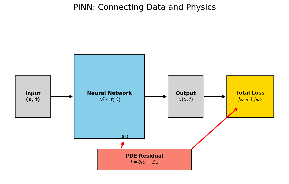
A neural network \(T_\theta(x,t)\) with a three-term loss:

\[ J = \underbrace{\frac{1}{N}\sum_i (T_\theta(x_i, t_i) - T_i^{\text{obs}})^2}_{J_{\text{data}}} \]

\[ + \lambda_{\text{PDE}} \cdot \frac{1}{M}\sum_j \left( \rho c_p \partial_t T_\theta - k\,\partial_{xx} T_\theta - q \right)_{(x_j,t_j)}^2 \]

\[ + \lambda_{\text{BC}}\, J_{\text{BC/IC}} \quad \text{(insulated edges, ambient at } t=0\text{)}. \]

PINN data flow: the network output feeds a data loss directly and, via automatic differentiation, a PDE-residual loss

Note

Collocation points \((x_j, t_j)\) are sampled densely between pyrometer pixels — that’s where physics supervises for free.

12. What the PINN buys you

• Spatial super-resolution: a smooth \(T(x,t)\) field where the pyrometer never measured (between pixels, between scan lines).

• Sub-frame time resolution: the network is differentiable in \(t\), so you can query \(T\) at arbitrary times beyond the 2 kHz camera grid.

• Derived fields for free: cooling rate \(\partial_t T\), gradient \(\partial_x T\) (drives solidification microstructure) — all from auto-diff on the same network.

Note

This is the PINN’s real value in the lab — not “we solved a PDE”, but “we obtained a quantity the sensor cannot measure”.

13. Inverse problem: estimate the absorptivity

• Effective absorptivity \(\alpha\) is a learnable scalar, optimised jointly with \(\theta\): \[ \min_{\theta, \alpha}\; J_{\text{data}}(\theta) + \lambda_{\text{PDE}}\, J_{\text{PDE}}(\theta, \alpha) + \dots \]
• The PDE residual disambiguates \(\alpha\): the only \(\alpha\) that makes \(J_{\text{PDE}} \to 0\) for the observed temperatures is the physical one.
• Compare to a Bayesian inverse: PINN gives a point estimate, but is dramatically cheaper than MCMC over a forward solver.

• Lab consequence: a single laser-power calibration sweep yields \(\alpha(P)\) across the operating envelope.
• Powder bed evolves over a build — refit \(\alpha\) per layer to track in-situ drift.

Note

One learnable scalar in the loss turns the PINN into a cheap inverse solver for material parameters.

14. What goes wrong: gradient pathology

• Reported by Wang, Teng & Perdikaris (2021): in many PINN setups the gradient of \(J_{\text{data}}\) (small, well-scaled) is dominated by the gradient of \(J_{\text{PDE}}\) (orders of magnitude larger).

• Symptom in the LPBF case: the network solves a PDE that satisfies the BCs but ignores the pyrometer. Predicted \(T\) is smooth but uncalibrated.

• Or the opposite: data dominates, PDE residual is ignored, predictions interpolate between pixels with no physical regularity.

Warning

A PINN that looks smooth but ignores the sensor has not failed loudly — inspect the gradient scale of both loss terms before trusting it.

15. Practical recipe

1. Log-transform losses before summing: \(\log J_{\text{data}} + \log J_{\text{PDE}}\) keeps both on the same scale.

2. NTK-based reweighting (Wang 2021): rescale \(\lambda_{\text{PDE}}\) at every step using the ratio of NTK traces of each loss term.

3. Curriculum: train \(J_{\text{data}}\) alone for \(\sim 10^3\) steps, then ramp \(\lambda_{\text{PDE}}\). The data fit “anchors” the network so the PDE residual has something to reduce.

4. Non-dimensionalise: rescale \(x \to x/L\), \(t \to t/\tau\), \(T \to T/T_0\) — turns the PDE coefficients into \(\mathcal{O}(1)\) Péclet/Stefan numbers and directly addresses scale mismatch.

Note

Non-dimensionalise first — it is the cheapest fix and often removes the pathology outright.

§D · Beyond PINN — Neural-operator surrogates

16. Beyond PINN — Physics-Informed Neural Operators (PINO)

• A vanilla PINN is trained on a single PDE instance: one set of boundary conditions, one source term, one geometry. Change any of those and you re-train.
• For a family of PDE problems (parametric BCs, swept geometries, varying source terms), the right object to learn is the solution operator \[ \mathcal{G}_\theta : \text{inputs} \;\longmapsto\; \text{solution field}. \]
• Neural operators (FNO; Li et al. 2020) learn \(\mathcal{G}_\theta\) directly: trained once, then evaluated on any new instance in milliseconds.
• PINO (Li et al. 2024) = FNO + the PINN residual loss. The operator both fits training solution pairs (data loss) and satisfies the PDE residual at sampled collocation points (physics loss).

• LPBF thermal-field prediction: train PINO once on simulated \((P, v, \text{geometry}) \to T(x,t)\) tuples; deploy on novel build geometries with no re-solve of the heat equation.
• Inference: milliseconds per build vs. minutes per FEM run — a regime change for in-loop process control.
• Same trick generalises to any parametric PDE the group already solves with FEM: thermal, diffusion, linear elasticity, phase-field.

A plain network on \(x(t)\) (a) vs. a network fed both \(x(t)\) and its Fourier transform \(\mathcal{F}[x(t)]\) (b) — the Fourier-input idea behind FNO layers

30-second derivation: an FNO layer replaces the kernel integral \(\int K(x,y)\,u(y)\,dy\) with a learned multiplication in Fourier space — FFT, point-wise complex weight, inverse FFT. The PINN residual is then computed on the output field of the operator. Why this composes cleanly: the operator is differentiable w.r.t. its inputs, so \(\partial_t u\) and \(\nabla^2 u\) at collocation points are just autodiff outputs of the operator forward pass. Anti-pattern: applying PINO to geometries far outside the training set — like any operator method, it extrapolates poorly; the PDE residual buys some regularization but does not turn a finite operator class into a universal solver. MFML W13 cross-reference: the PINO slide there derives the Fourier-layer math; here we just consume the result.

17. GNN PDE Solvers — MeshGraphNets for Irregular Materials Meshes

• FNO assumes a regular grid (FFT lives there). Many materials problems do not: polycrystalline grain-boundary networks, finite-element meshes for composite micromechanics, foamed-cell topologies — these all live on irregular meshes.
• MeshGraphNets (Pfaff et al. 2021) (Pfaff et al. 2021) treat the mesh as a graph: nodes carry physical state (displacement, temperature, stress), edges carry connectivity, and a GNN learns local message-passing updates that approximate one PDE time-step.
• Trained once on a few thousand FEM-simulated mesh / field pairs; generalises across meshes of different sizes and topologies.

• Materials use case: predict stress fields on a polycrystal grain network without solving the elasticity FEM each time.
• Training data: a few \(10^3\) FEM-simulated grain meshes plus their stress fields.
• Inference: one GNN forward pass, \(\mathcal{O}(\text{edges})\) — fits the inner loop of a microstructure-aware design optimisation.

Note

FNO needs a grid; when the physics lives on an irregular mesh, message passing is the operator.

One message-passing step (the recipe): (i) edge update — each edge embedding is a learned function of its two endpoint node states and any static edge features (rest-length, normal); (ii) aggregate — each node sums (or means) the incoming edge messages; (iii) node update — each node embedding is a learned function of its old state and the aggregated message. Stack a handful of these steps and you have one PDE update. Why this beats FNO on irregular meshes: FNO needs a regular grid for the FFT; a GNN is grid-free by construction. Accuracy bar reported in the literature: GNN solvers reach FEM-level RMSE with roughly an order-of-magnitude shorter training-to-inference cycle. MFML W13 reference for the GNN-layer math. Anti-pattern: train on tetrahedral solid meshes, deploy on a triangulated foam — different topology class, expect generalisation to fail. 1080Ti budget: comfortably handles \(\sim 10^4\)-node meshes in training; larger meshes need gradient checkpointing or mini-batching by sub-graph.

§E · Pattern C — Symmetry-aware NN for the elastic tensor

18. Setup: predict Cᵢⱼ from a structure descriptor

• Target: full \(6 \times 6\) Voigt elastic tensor \(C_{ij}\) for an unseen composition.
• Inputs: descriptor of the crystal — composition vector, lattice parameters, Wyckoff positions, or a graph of atoms.
• Hard constraint: \(C_{ij}\) must respect the point-group symmetry of the crystal.

• For cubic crystals only 3 of 21 components are independent; for hexagonal, 5; for triclinic, all 21.
• A naive NN that outputs 21 numbers will always break symmetry on novel inputs unless told otherwise.

Note

Symmetry decides how many of the 21 components are real degrees of freedom — the network should not have to rediscover that from data.

19. Two paths to enforce symmetry

Path 1 — symmetry-augmented training.

• For every training crystal, apply each point-group operation \(g\) (rotation, reflection, inversion).
• Train on the augmented dataset: input \(g \cdot \text{descriptor}\), target \(g \cdot C_{ij}\).
• Effort: a data-loader change. Implementation cost: small.

Path 2 — equivariant network architecture.

• Use an architecture (NequIP, e3nn) whose layers are equivariant by construction: \[ f(g \cdot x) = g \cdot f(x) \quad \forall g \in G. \]
• Output is a tensor of the correct rank that automatically transforms correctly under \(G\).
• Effort: architectural — tensor-product layers and Clebsch–Gordan coefficients.

Note

Same constraint, two prices: a data-loader change buys you approximate symmetry; an equivariant architecture buys you exact symmetry.

20. Trade-off: easy vs. exact

Augmentation (Path 1)

• Pros: drop-in, any backbone works, easy to debug.
• Cons: only approximate symmetry — depends on data coverage. Symmetries away from training distribution are not guaranteed.
• Cost at inference: same as the base model.

Equivariant net (Path 2)

• Pros: exact symmetry, by construction.
• Cons: harder to engineer; tensor types and irreducible representations bookkeeping. Slower per parameter.
• Cost: typically 2–5× per forward pass vs. an MLP of the same width.

Note

Pick by deployment scenario. Screening 10\(^5\) candidates? Augmentation. Generating training data for a downstream physics simulator that requires exact symmetry? Equivariant.

21. What it enables

• Predict full \(C_{ij}\) from a Materials Project descriptor for compositions where DFT is too expensive (high-throughput screening, \(10^5\)+ candidates).

• Downstream: derive bulk modulus \(K\), shear modulus \(G\), anisotropy ratio, sound velocities — all from \(C_{ij}\) — without ever running ab-initio.

Note

The symmetry constraint is what makes the predictions trustworthy enough to feed into the next stage of an inverse-design loop, instead of being treated as unverified guesses.

§F · Pattern D — Physics-regularized time series for process drift

22. Setup: in-situ stress–strain during forming

• Streaming inputs from a forming press: load cell (\(\sigma_t\)), displacement (\(\epsilon_t\)), torque, optionally acoustic emission.
• Goal: real-time prediction of the yield event — the moment the workpiece transitions from elastic to plastic.
• Latency budget: a few ms per inference (control loop closes at 1 kHz).

• Sequence model: 1D-CNN or small Transformer over a sliding 100 ms window.
• Output at each step: \(p(\text{yield})\) plus a calibrated stress estimate.

Note

A 1 kHz control loop leaves a few milliseconds per inference — the latency budget constrains the model as hard as the physics does.

23. The constraints to enforce

• Monotonic loading: while the actuator is loading, \(\epsilon_t\) only increases until an explicit unload.

• Positive stiffness in the elastic regime: \[ \frac{d\sigma}{d\epsilon} > 0 \qquad \text{for } \epsilon < \epsilon_y. \]

• Graceful sensor dropout: the model must degrade smoothly when one of \(\{\sigma, \epsilon, \tau\}\) drops out — the underlying mechanical state is still observable from the others.

Note

All three constraints are statements about the physical state, not about any single sensor — that is what makes them enforceable.

24. How to enforce monotonicity

Structural (hard). Predict cumulative non-negative increments and integrate: \[ \Delta\sigma_t = \text{softplus}\,\big(\text{NN}(x_t)\big) \ge 0, \qquad \sigma_t = \sigma_0 + \sum_{s \le t} \Delta\sigma_s. \]

Monotonicity is now exact. A non-negative output activation is a tiny architectural change with a hard guarantee.

Soft. Penalize negative slope inside the elastic region: \[ J_{\text{mon}} = \lambda_m \sum_{t : \epsilon_t < \epsilon_y} \max\!\left(0,\, -\frac{d\sigma_\theta}{d\epsilon}\right)^2. \]

Easier to add, but only approximate; behaves badly near the yield transition where the indicator function is itself uncertain.

Note

When a hard structural guarantee costs one activation function, take it.

25. Sensor dropout — physics-aware augmentation

• Train with random masking over input channels: at each step independently set \(\sigma_t = 0\) (or \(\epsilon_t = 0\), \(\tau_t = 0\)) with probability \(p\).

• Verify on held-out test runs that masking any one of the three channels degrades RMSE by < 10% — i.e. the model genuinely uses the redundancy.

• Why “physics-aware”: the underlying mechanical state is observable from any one of several physically equivalent signals. The masking does not invent redundancy that isn’t there — it forces the network to use redundancy that is.

Note

Masking only works because the physical redundancy is real — verify the < 10% degradation on held-out runs; don’t assume it.

§G · What still goes wrong

26. Constraint conflicts

• Physics says \(A \ge 0\). Data says \(A < 0\).

• This almost always means one of:
  • Systematic measurement error (calibration drift, sign convention, detector zero).
  • The physics model is wrong / incomplete in this regime (e.g. a phase transition you didn’t put in the equation).
  • Data leakage — labels actually come from a different signal than you think.

Warning

Don’t suppress the conflict by raising \(\lambda\). Diagnose it. The conflict is a free signal that something upstream of the model is broken.

27. Loss-weight tuning pain

• Gradient pathology (Wang 2021): one loss term dominates the gradient by orders of magnitude.

• Scale mismatch: \(J_{\text{data}}\) in \(K^2\), \(J_{\text{PDE}}\) in \((K/s)^2\) — same number, totally different physical magnitudes.

• Tools that help, in increasing order of effort:
  • Non-dimensionalise the PDE first.
  • GradNorm — adapt \(\lambda\) so each loss term contributes equally to the gradient norm.
  • NTK-based reweighting (Wang 2021).
  • Multi-objective optimisation — Pareto fronts over \((J_{\text{data}}, J_{\text{phys}})\).

Note

Work up the effort ladder — non-dimensionalise, then GradNorm, then NTK reweighting; most lab cases never need the top rung.

28. When constraints become crutches

• If the model only works with a hand-coded constraint and collapses without it — the architecture is wrong, not under-constrained.

• Constraints should help generalization, not patch a flawed model. A symptom: removing the constraint produces nonsense (negative grain sizes, energy explosion). A diagnosis: the model has no inductive bias toward the right kind of function in the first place.

• Counter-example: a CNN with the wrong receptive field cannot be saved by a soft-monotonicity penalty — it never sees the temporal context that makes monotonicity meaningful.

Warning

If removing the constraint produces nonsense, the constraint is masking an architecture bug — fix the model, not \(\lambda\).

29. Pointer to MFML W13 (taught Mon 13.07 — after this unit)

Note

For the math behind the patterns we used today:

• PINN loss derivation, AD, collocation theory — MFML W13 §6–8.
• Lagaris substitution for hard BCs — MFML W13 §9.
• DeepONet & FNO architectures — MFML W13 §12.
• Equivariant networks, Hamiltonian NNs — MFML W13 §12.
• SINDy and equation discovery — MFML W13 §6.

Today we used the results. The derivations live there.

§H · Wrap

30. Recap: Unit 11

1. Pick the right pattern per task: soft constraint (Pattern A), full PINN (B), neural-operator surrogate (PINO / MeshGraphNets) when you need a family of PDE instances, symmetry architecture (C), structural monotonicity + masking (D).

2. Constraints help generalization — they do not patch a broken architecture. If you cannot remove the constraint without nonsense, fix the model.

3. Calibrate the data–physics trade-off explicitly: report data error and constraint-violation rate as separate axes.

4. MFML W13 has the math; this unit is the playbook for using it on real instruments.

Continue

• ← Previous: Unit 10 — Transformers for materials characterization (ViT, Flash Attention, Mamba)
• → Next: Unit 12 — Uncertainty-aware regression & Gaussian Processes
• All courses

31. References & further reading

• Raissi, Perdikaris, Karniadakis (2019): Physics-Informed Neural Networks. J. Comp. Phys. 378.
• Wang, Teng, Perdikaris (2021): Understanding and mitigating gradient pathologies in PINNs. SIAM J. Sci. Comp.
• Lagaris, Likas, Fotiadis (1998): ANN methods for ODE/PDE BC substitution. IEEE TNN 9(5).
• Lu, Jin, Karniadakis (2021): DeepONet — learning nonlinear operators. Nat. Mach. Intell. 3.
• Batzner et al. (2022): NequIP — equivariant graph NN for interatomic potentials. Nat. Comm. 13.
• Karniadakis et al. (2021): PIML overview. Nat. Rev. Phys. 3.
• Neuer (2024): Ch. 6 — Physics-Informed Learning (lab perspective).
• LPBF / melt-pool PINNs: Liao et al. (2023); Zhu et al. (2021) — heat-equation PINNs for AM.

Li, Zongyi, Hongkai Zheng, Nikola Kovachki, et al. 2024. “Physics-Informed Neural Operator for Learning Partial Differential Equations.” ACM/IMS Journal of Data Science 1 (3): 1–27.

Pfaff, Tobias, Meire Fortunato, Alvaro Sanchez-Gonzalez, and Peter W. Battaglia. 2021. “Learning Mesh-Based Simulation with Graph Networks.” International Conference on Learning Representations (ICLR).