Machine Learning for Characterization and Processing
Unit 12: Uncertainty-aware regression & Gaussian Processes

AI 4 Materials / KI-Materialtechnologie

Prof. Dr. Philipp Pelz

FAU Erlangen-Nürnberg

§A · From MFML theory to lab practice

01. MFML W12 recap — we use these, we do not re-derive them

Method	One-line summary	When to reach for it
Gaussian Process	Closed-form Bayesian regression over functions	Small \(n\) (\(\lesssim 10^3\)), tabular, smooth response, need calibrated CI
MC Dropout	Keep dropout on at inference, sample \(T\) passes	Big NN already trained, cheap epistemic estimate per pixel/voxel
Deep ensembles	Train \(M\) independent NNs, use disagreement	Best-calibrated NN UQ; budget for \(M\times\) training
MDN	NN outputs \((\pi_k, \mu_k, \sigma_k)\) of a Gaussian mixture	Multi-modal output (phase A or phase B from the same input)
Calibration	Reliability diagram + temperature scaling	Mandatory before any deployed model

Note

We are not re-deriving the math. See MFML W12 for posteriors, ELBO, marginal likelihood. Today: which tool, on which lab task, with which numbers.

Framing for the unit. This is a deployment-and-decisions unit, not a derivation unit. Students arrive here with the MFML W12 math in their notebooks already (GP posterior, ELBO, marginal likelihood). My job today is to turn that math into instrument-time saved, scrap rate avoided, and acquisition functions that pick the next experiment. If a student raises a hand to ask “where does the GP posterior come from?”, point at MFML W12 and keep moving.

Use this table as a navigation index. Every row is a slide later in the deck — GP in §3, MC Dropout in §4, ensembles + MDN in §6, calibration as the backbone in §6. When students get lost in the deck, return to this table.

Anti-pattern to flag early. Most published materials-ML papers ship a model with a softmax score and call it “confidence”. The whole point of this unit is to make students physically uncomfortable with that practice, so they go fix it on their own projects. Plant that discomfort here.

Pacing. This slide opens the unit and should land in under 90 seconds — it’s a map, not a lesson. The lesson starts on the next slide.

Cross-reference. MFML W12 is the math backstop; ML-PC u06 (DINOv2 transfer) is where overconfident foundation models first bite; ML-PC u09 (spectra) is where calibration on small spectroscopy datasets is non-negotiable.

02. Why UQ matters in characterization & processing labs

• One wrong tensile-strength call on a structural part: recall, scrap, or worst case a failure in service.
• One missed crack/pore in an SEM screen: a defective batch ships.
• A point estimate without a confidence band is not a deliverable to a lab manager or a certifying body.

• Engineering decisions are threshold decisions — accept/reject, retest/release, explore/exploit.
• A threshold needs a distribution, not a number.

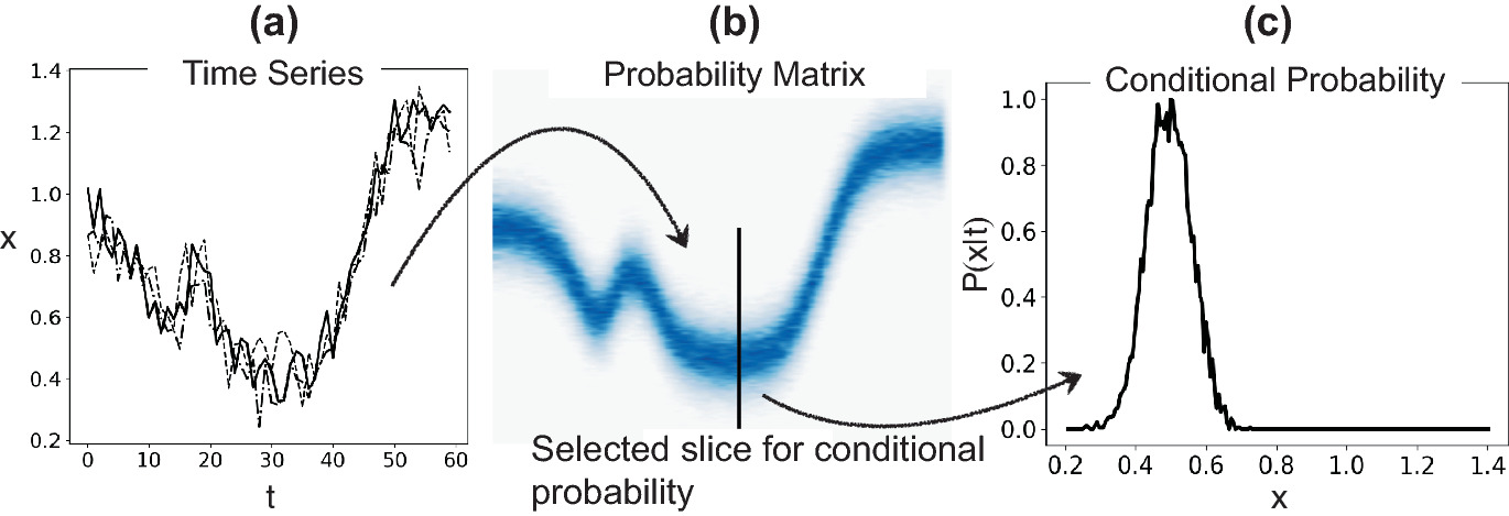
A probability corridor around a process signal: the conditional distribution \(p(x\,|\,t)\) — not a point estimate — is what a threshold decision reads off.

Note

Trust = prediction + calibrated confidence. The “calibrated” word is what most published materials-ML papers skip.

Why this slide is the emotional anchor. Engineering decisions are threshold decisions — accept/reject, retest/release, explore/exploit. A threshold needs a distribution, not a number. Until students feel that, they will keep reporting RMSE without a confidence band on their MSc projects. Spend a full minute on the “not a deliverable” line.

Concrete story to use. I usually retell a specific scrap incident: a hardness model with no uncertainty band predicted a tempered part inside spec; the part shipped, failed in service on a customer rig, and the recall cost six figures. The fix afterwards was not a better mean predictor — it was adding a CI and a hard reject rule above a width threshold. Same model, different deployment, opposite outcome.

Anti-pattern. Students will read papers reporting “test accuracy 97 %” and call that “trust”. Push back: 97 % marginal accuracy with the failures concentrated in the high-confidence tail is worse than 92 % with well-distributed mistakes. Trust requires the shape of the error distribution, not its mean.

Cross-reference. ML-PC u02 (physics-of-data) introduced “all measurement is noisy”; this slide finishes that thread — noise is not a nuisance to absorb, it is the signal the model must propagate.

Pre-empt. “Is this just for safety-critical parts?” — no. UQ is the input to the next experiment (§5). Even when the part is non-critical, your budget is critical, and a calibrated \(\sigma\) is what picks the next experiment.

Pacing. ~2 minutes. Land the threshold framing before moving on.

03. Two pain points unique to materials labs

(a) Tool / operator / coating domain shift

• The training set was acquired on SEM #1 with operator A and a 5 nm Au coating.
• Inference happens on SEM #2, operator B, no coating, on Tuesday after a chamber vent.
• Your softmax does not know any of that. Your uncertainty had better grow.

(b) Experiments cost €1k+/h

• Analytical S/TEM, AM build chambers, Gleeble dilatometry: each new label is hours of instrument time and days of prep.
• UQ is not a publication ornament — it is the input to the next experiment: active learning only works if uncertainty is honest and spatially resolved.

Warning

A model that gets quieter as the input drifts is broken — under tool, operator, or coating shift your uncertainty must grow.

Both pain points are materials-specific. Web-scale ML papers do not have either: their distribution shift is a covariate-shift benchmark, and their next “experiment” is another web crawl at marginal cost. Drive that contrast home — the reason our subfield needs honest UQ is that experiments are expensive and instruments drift.

Pain point (a) — domain shift. The realistic deployment of any materials model is on a different tool, by a different operator, with a different prep. Most softmax-based models cannot tell. Today’s unit is about models that can tell — either by ballooning \(\sigma\) (GP, ensemble), by entropy spikes (MC Dropout), or by OOD detectors (Mahalanobis, §6). A model that gets quieter as the input drifts is broken; you want one that gets louder.

Pain point (b) — €1k+/h experiments. This is the slide that motivates §5 (active learning) and §3’s ROI. A tensile + hardness round at €200/test is cheap by materials standards; analytical S/TEM is closer to €500-1000/h once you add operator + amortised instrument cost. Make the numbers concrete so students do not dismiss them as toy.

War story. I have seen a PhD project waste six months because a CNN was retrained from scratch every time a new SEM was added — there was no calibration step, so the team assumed the model itself was the problem. The model was fine. The calibration was missing.

Cross-reference. Pain point (a) → §6 (calibration on lab-realistic sets, OOD detectors); pain point (b) → §5 (AL loop). The whole deck is structured around these two failure modes.

Pacing. ~2 minutes. Two halves, one each. Move on quickly to §2 (method selection).

§B · Picking a UQ method per lab task

04. Decision table — task → method → cost

Lab task	Recommended UQ	Rationale	Cost driver
Tabular regression, \(n \in [10, 300]\) (composition \(\to\) property)	GP, RBF or Matérn \(\nu{=}5/2\)	Closed-form CI, smooth response, hyperparams interpretable	\(O(N^3)\) once — fine for \(N \lesssim 10^3\)
Pixel-wise segmentation of microscopy (CNN, U-Net)	MC Dropout, \(T \approx 30\)	Reuse trained net, get per-pixel variance map	\(T\times\) inference per image
High-stakes property regression with budget for retraining	Deep ensemble, \(M \in [5, 10]\)	Best calibration in literature (Lakshminarayanan et al. 2017)	\(M\times\) training
Multi-modal output (one input, two phases possible)	MDN, \(K \in \{2,3\}\)	Bimodal \(p(y\|x)\) — mean is meaningless	One training, harder to fit
Any deployed model	Reliability diagram + temp scaling	Free, post-hoc, on a held-out cal set	Trivial

Note

Every row except the MDN is post-hoc — you can bolt it onto an already-trained model. The calibration row is mandatory on top of all the others.

This is the slide students will photograph. Make sure the four cost drivers are named, not just hinted at: \(O(N^3)\) (GP), \(T\times\) inference (MC Dropout), \(M\times\) training (ensemble), one-off fit (MDN). Each is a different bottleneck and dictates a different deployment story.

Materials hook for each row. GP row → tabular composition→property (§3); MC Dropout row → SEM segmentation (§4); ensemble row → high-stakes property prediction (e.g., yield strength for a structural alloy spec) — same model trained 5× and disagreement is the signal. MDN row → phase-field outputs where the same composition can crystallise into two phases; the mean is a meaningless intermediate composition and a single Gaussian undersells the multi-modality.

Anti-pattern. Choosing the model first and forcing UQ on afterward. The right order is (a) what is the prediction task and noise model? (b) which UQ family fits? (c) which model in that family? Walking from prediction-task to method is the whole point of this slide.

Pre-empt. “Why not Bayesian NNs / variational inference?” — defer to MFML W12 and to the textbook Murphy ch.4. In practice, ensembles dominate them for materials-scale problems on calibration and engineering simplicity. We mention BNNs only if a student raises them.

Materials-meta observation. Every row except MDN is post-hoc applicable — you can bolt it on top of a model that was trained without UQ in mind. MDN bakes UQ into the loss and the architecture, so it has to be a planned choice from day one. That asymmetry matters for retrofitting existing models on your team.

Forward link. §6 (calibration + temp scaling) is the bottom row and is mandatory, not a “nice to have”. Every other row needs calibration on top.

05. Materials-specific computational budgets

Training-time vs inference-time tradeoff is more loaded in a lab than in webscale ML:

• Deep ensemble — cheap at inference (run \(M\) small NNs, average), expensive at training (\(M\times\) wall-clock + carbon). Acceptable when training is one-off and the model is shipped to many labs.

• MC Dropout — cheap at training (one network), expensive at inference (\(T\times\) forward passes). Acceptable on a benchtop where you process tens of images per day; not acceptable for a real-time inline detector.

• GP — both small at the scales we operate (\(N \lesssim 1000\)). Recompute per dataset; trivially cheap at inference.

Warning

MC Dropout’s variance estimate degrades with very deep nets and very low dropout rates — it can collapse to near-zero variance and look overconfident. Always validate with a held-out reliability diagram.

Carbon-budget angle. A 5-member ensemble of ResNet-50 trained from scratch is ~5× the embodied carbon of a single model. For models that ship to many labs (foundation models, certified analyzers) this amortises; for in-house ad-hoc projects it does not. Push students to think about who pays the training cost vs who pays the inference cost.

Real-time-detector nuance. Inline SEM defect spotters running at video rate cannot afford 30 forward passes per frame. MC Dropout is then the wrong tool — either accept ensembles (parallel inference, expensive in VRAM) or drop to a single deterministic net + post-hoc calibration. Students who skip this step ship overconfident inline detectors.

The callout-note is load-bearing. MC Dropout’s variance is not a guaranteed posterior — it is an interpretation under the variational-approximation assumption of Gal & Ghahramani. In modern architectures (deep, low dropout, batchnorm everywhere) that interpretation gets shaky. The fix is always a held-out reliability diagram, not a different formula.

Anti-pattern. Using a wall-clock argument to justify the wrong UQ choice. (“We chose MC Dropout because it was 1 day to wire up.”) Wall-clock matters at deployment, not at justification. Pick by task; pay for it.

Pre-empt. “Why does GP scale as \(N^3\)?” — Cholesky of the \(N \times N\) kernel matrix. We do not re-derive in class; pointer to MFML W12.

Cross-reference. This pairs with the next slide (§2 “What to not do”) which is the negative version of the same advice.

06. What to not do

• Do not quote raw softmax probability as “model confidence” — modern deep nets are systematically overconfident; a 0.97 softmax on an out-of-distribution micrograph is meaningless (Guo et al. 2017).

• Do not report the variance of a single ensemble member’s Monte-Carlo dropout passes and call it ensemble uncertainty — you are mixing two distinct UQ techniques and double-counting.

• Do not report a GP fit without showing the prior (kernel choice, length-scale prior). The kernel is the model. Hiding it makes the CI uninterpretable.

• Do not report any UQ number without a reliability diagram on a held-out calibration set.

Warning

All four anti-patterns share the same antidote: a reliability diagram on a held-out, lab-realistic calibration set.

This is the “be ashamed if you do this” slide. Read each bullet slowly. Each one corresponds to a published paper I can name (and so can the students after this slide if they pay attention to their next literature review).

Bullet 1 — softmax-as-confidence. Modern deep nets are systematically overconfident; the standard literature on this is Guo et al. 2017, but the materials-specific failure mode is OOD micrographs (different tool, different coating). A 0.97 softmax on an in-distribution image and a 0.97 softmax on an OOD image look identical to the user. The fix is calibration + OOD detection (§6) on top, not a different network.

Bullet 2 — single-member MC dropout variance. This is a category error — combining “an ensemble member” with “MC dropout passes” gives a meaningless mixed estimator. Either pick one or compose them properly (run MC dropout for each ensemble member and pool). Most thesis projects make this mistake at least once.

Bullet 3 — GP without kernel. A GP fit reported without its kernel (and length scale prior) is unfalsifiable. The kernel is the model. If a paper shows a GP curve without telling you whether they used RBF or Matérn 5/2, what \(\ell\), what \(\sigma_n\), treat the CI as advertisement, not evidence.

Bullet 4 — no reliability diagram. Same flavour as bullet 3. UQ numbers without coverage diagnostics are decoration. We will keep returning to this throughout §6.

Pacing. ~2.5 minutes. The four bullets are punchlines; do not over-explain — let students feel the discomfort.

War story. Tell the class about a recent reviewer-2 incident: a paper claiming “uncertainty-aware” did all four anti-patterns simultaneously. Reviewer 2 (me) sent it back with a single rejection: Add a reliability diagram on a held-out lab-realistic set.

Forward link. §6 deals with how to not commit these anti-patterns; §3-5 are the constructive examples.

§C · Case study A — GP for process→property mapping

07. Setup: 21CrMoV5-7 quench-and-temper

• Steel grade DIN 1.7709 / 21CrMoV5-7 (Mantzoukas et al. 2021).
• Process: austenitize 960 °C / 30 min, oil quench, temper 2 h at variable \(T_{\text{temper}}\).
• Input: \(T_{\text{temper}} \in \{475, 500, 525, 550, 575\}\) °C.
• Output: hardness HV30 (six indents per specimen, averaged); \(379\text{–}409\) HV30 \(\approx 38.7\text{–}41.7\) HRC.
• Real published dataset: 5 temperatures × 10 specimens = 50 values, published to the last indent (Table 3 of the paper; data_mantzoukas2021_table3.csv).

Why this is a textbook GP problem:

• \(n\) small, \(d{=}1\) input, real cost per specimen.
• Response is not monotonic: secondary-hardening peaks at 500 and 550 °C (Cr/Mo/V carbide precipitation) — a parametric “softening curve” fit would be wrong.
• 10 replicates per condition → the noise level \(\sigma_n\) can be estimated from the data, independent of the model.

Note

Small \(n\), one physical input, replicate scatter, non-trivial shape — the textbook regime for a GP.

Why this alloy, why this data set. 21CrMoV5-7 (DIN 1.7709) is a workhorse Cr-Mo-V quench-and-temper steel for pressure-vessel and rotor applications — and the Mantzoukas et al. 2021 paper (MATEC Web Conf. 349, 02005, open access) publishes the complete raw data: 50 randomized specimens from one bar batch, five tempering groups, every HV30 value in Table 3. Everything on the next four slides is computed from that table — the CSV and the fitting script (make_gp_figures.py) are in the unit folder, so students can reproduce every number.

Physics in one breath. In plain-carbon steels tempering monotonically softens. Not here: in Cr-Mo-V grades the 475-575 °C window is exactly where secondary hardening happens — Cr/Mo/V alloy carbides precipitate and re-strengthen the matrix, competing with the recovery of the martensite. The measured response is nearly flat overall (379-409 HV30) with peaks at 500 and 550 °C. The paper’s own conclusion: the grade “resists tempering back” in this window. This non-monotonic fine structure is the whole reason a parametric softening law fails and kernel choice (next slide) matters.

Why the group means are trustworthy. 10 replicates per condition, each specimen itself the mean of six HV30 indents, all specimens randomized from one batch (Minitab randomization, one furnace). Standard error of a group mean ≈ \(\sigma_n/\sqrt{10} \approx 4\) HV30 — so the 500 °C peak (409 vs 381 at the neighbours) is a ~7-SE effect, unambiguously real signal, not noise.

Why \(n = 50\) is still “small data”. Fifty scalar measurements is far too small for any neural network to give honest uncertainty, and exactly the regime where a GP shines. Also note the heteroscedasticity in Table 3: group SDs run from 4.6 (575 °C) to 20.2 HV30 (500 °C) — precipitation-driven scatter. We fit a homoscedastic GP with the pooled SD and flag the heteroscedastic extension in the notes of slide 09.

Anti-pattern. Students will try to fit a polynomial regression with bootstrapped CIs. On this data a low-order polynomial averages away the two secondary-hardening peaks and a high-order one chases the noise. The GP is the right tool because it has a principled prior (correlation length) and a principled posterior CI.

Cross-reference. Mantzoukas_2021_17709 in ref.bib; full PDF in the unit folder. MFML W12 for the posterior derivation. ML-PC u02 (physics-of-data) for the discussion of replicate scatter vs model uncertainty.

Pacing. ~1.5 minutes. The setup is short — the lecture should move quickly to the kernel slide.

08. Why GP fits this lab task

• \(n = 50\): too small for a deep net to give honest uncertainty, plenty for a GP.
• Matérn \(\nu{=}5/2\) encodes “smooth response with a finite correlation length” — the right inductive bias for precipitation kinetics.
• The GP delivers what the lab manager wants: \(\hat{y}(T) \pm 2\sigma(T)\), narrowing at sampled \(T\), widening between.

• Fitted to Table 3: \(\sigma_n = 13.4\) HV30 fixed from the replicates; \(\sigma_f = 13\) HV30 by maximum likelihood; \(\ell = 13\) °C by MAP (next slide). See MFML W12 for the marginal-likelihood formula — we use the result.

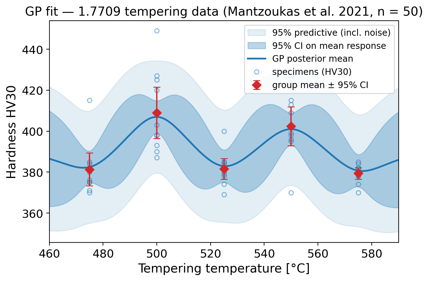
GP fit to the actual Mantzoukas Table-3 data (all 50 specimens): the CI on the mean response narrows at the five sampled temperatures and widens between them; the light band adds the replicate noise.

Note

At \(n = 50\) the GP’s posterior CI is honest by construction — the leave-one-out check on this fit gives 92% empirical coverage for the 95% band (slide 10).

Three reasons GP wins here, in plain words. 1. Small-data calibration: with \(n = 50\) the GP’s posterior CI is honest by construction — no need for a separate calibration set. Neural-net UQ at \(n = 50\) is fantasy. And we check the construction: leave-one-specimen-out coverage on this fit is 46/50 = 92% for the nominal 95% band (slide 10). 2. Correlation-length prior: Matérn 5/2 encodes “the response varies smoothly with a characteristic temperature scale” — exactly the inductive bias precipitation kinetics gives you for free. Note it does not assume monotonicity, which is what saves us here. 3. Interpretable hyperparameters: \(\ell\) is a characteristic temperature scale the metallurgist can read — here 13 °C, i.e. the secondary-hardening peaks are narrower than the 25 °C sampling grid. Try explaining a 100-parameter MLP’s hidden activations to your lab manager.

Walk the figure. All 50 raw specimens (open circles), group means ± 95% CI (red diamonds), GP posterior mean, dark band = 95% CI on the mean response, light band = predictive interval including replicate noise. Point at the 449 HV30 specimen at 500 °C: a genuine outlier the paper kept; the predictive band absorbs it, the mean band does not chase it.

Why we do not derive the marginal likelihood. It is a one-liner: \(\log p(y \mid X, \theta) = -\tfrac{1}{2} y^\top K_\theta^{-1} y - \tfrac{1}{2}\log|K_\theta| - \tfrac{n}{2}\log 2\pi\). The two terms balance data fit against model complexity — automatic Occam’s razor. We use this; MFML W12 derives it.

Pre-empt. “Why not just bootstrap the data and fit polynomials?” — bootstrap CIs are empirical, not predictive; they do not widen between data points. GP is the right tool because the CI grows where there is no data and shrinks where there is.

Materials-specific pre-empt. “Why not a physics-based parametric model (Hollomon-Jaffe parameter)?” — Hollomon-Jaffe assumes monotonic tempering-back and cannot represent secondary hardening at all; on this alloy it is structurally wrong in exactly this window. The defensible hybrid is Hollomon-Jaffe (or any parametric softening law) as the GP’s prior mean with the GP correcting deviations — mention that the hybrid exists; here the non-parametric GP alone is the honest choice.

Cross-reference. MFML W12 for the marginal-likelihood objective and the Cholesky-based solver; ML-PC u11 (PINNs, the previous deck) for the physics-prior hybrid.

Pacing. ~2 minutes.

09. Kernel choice — what the hyperparameters mean physically

\[ k_{\text{RBF}}(T, T') = \sigma_f^2 \exp\!\left(-\frac{(T - T')^2}{2\,\ell^2}\right) \]

• Length scale \(\ell\): the “characteristic process variability” on the temperature axis.
  • Fitted here: \(\ell \approx 13\) °C → the secondary-hardening peaks are narrower than the 25 °C sampling grid.
  • \(\ell \approx 200\) °C → prior samples are near-straight trends; the peaks at 500/550 °C are oversmoothed away.

• Signal variance \(\sigma_f^2\): amplitude of the hardness variation across the window — fitted \(\sigma_f = 13\) HV30, matching the \(\sim\) 30 HV30 peak-to-valley swing.

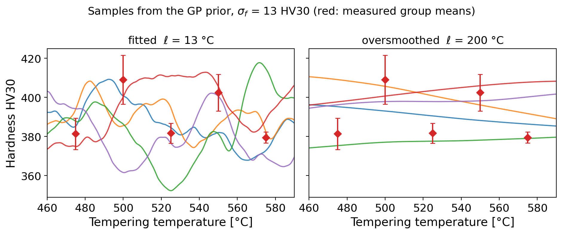
Samples from the GP prior with the hyperparameters fitted to the 1.7709 data (left) and with a deliberately oversmoothed length scale (right); red: the measured group means.

• Noise variance \(\sigma_n^2\): instrument + specimen scatter at fixed \(T\). Estimated from the 10 replicates per group and fixed: \(\sigma_n = 13.4\) HV30. Do not let the optimizer absorb model misfit into noise.

Note

For metallurgical responses with regime changes, prefer Matérn \(\nu{=}5/2\) over RBF — it is once-differentiable instead of \(C^\infty\), which matches the physics better.

The slide that distinguishes ML-PC from MFML. In MFML we taught the GP as math — kernels are positive-definite functions. Here, each kernel hyperparameter has a physical reading: \(\ell\) is a temperature scale, \(\sigma_f^2\) is the data range, \(\sigma_n^2\) is replicate scatter. If a student cannot give each hyperparameter a unit and a physical interpretation after this slide, they did not get the point.

Trap to flag explicitly: \(\sigma_n^2\) as a model-misfit sponge. If you let the optimiser pick all three hyperparameters freely, it will absorb model misfit (wrong kernel, wrong mean function) into \(\sigma_n^2\), blowing up the noise estimate. The right discipline — used for this actual fit — is to estimate \(\sigma_n^2\) from the replicates (pooled within-group SD of Table 3: \(\sigma_n = 13.4\) HV30) and fix it during marginal-likelihood optimisation. This single discipline change is the most common audit-fix I make on student GP code.

The second trap, which this data actually springs: degenerate \(\ell\) under free MLE. With 25 °C spacing and an up-down-up-down group-mean pattern, the marginal likelihood is nearly flat for all \(\ell\) below the grid spacing and the optimiser runs \(\ell \to 0\) (the “every condition is independent” limit). The fix is the one slide 11’s caveat preaches: an informative prior. We used \(\ell \sim \text{LogNormal}(\ln 25\,°\text{C}, 0.5)\) — centred on the sampling spacing — and took the MAP, landing at \(\ell = 12.6\) °C. Lesson: the data cannot resolve structure finer than its own sampling grid, and the hyperparameters will tell you so if you listen.

Heteroscedasticity footnote. Table 3’s group SDs range 4.6–20.2 HV30 (largest exactly at the 500 °C precipitation peak). We pool to a single \(\sigma_n\) for simplicity; the honest extension is a heteroscedastic noise model with per-group \(\sigma_n\) — good MSc-thesis exercise.

Why Matérn 5/2 for metallurgy. RBF is \(C^\infty\) smooth — every derivative exists. Real tempering responses have sharp features (here: secondary-hardening peaks barely wider than 25 °C). Matérn 5/2 is twice differentiable but not more — it can bend more sharply where the physics calls for it. Bishop ch.6 has the full kernel zoo.

Pre-empt. “Should I use ARD (one \(\ell\) per input dimension)?” — yes, always, when \(d > 1\). It is the cheapest interpretability win and it surfaces which inputs are irrelevant.

Anti-pattern. Reporting a GP fit without listing the hyperparameter values and how each was set. The reproducible statement for this fit is: “Matérn 5/2, \(\ell = 13\) °C (MAP, LogNormal prior at the 25 °C spacing), \(\sigma_f = 13\) HV30 (MLE), \(\sigma_n = 13.4\) HV30 (fixed from replicates)”. If a paper does not give you the equivalent sentence, treat its GP as unreproducible.

Cross-reference. ML-PC u12 (next unit, PINNs) builds on the prior-mean / kernel-prior structure.

Pacing. ~3 minutes — this is the GP-internals slide. Spend the time.

10. The fit — and its held-out test

• Posterior mean: flat around 380 HV30 with two secondary-hardening peaks (407 at 500 °C, 401 at 550 °C).
• 95% CI ribbon on the mean: tight (\(\pm 8\) HV30) at the five sampled tempers, widens to \(\pm 19\) HV30 mid-gap — the ribbon breathes with the data.
• Leave-one-specimen-out check on the full fit: 46/50 = 92% of specimens inside the nominal 95% predictive band.

Held-out check (figure). Refit with the entire 525 °C group hidden: the GP predicts \(399 \pm 26\) HV30 (95%) there; the hidden group measured \(382 \pm 5\) — inside the band. The interval is wide because the neighbouring peaks make interpolation genuinely uncertain. That width is information, not weakness.

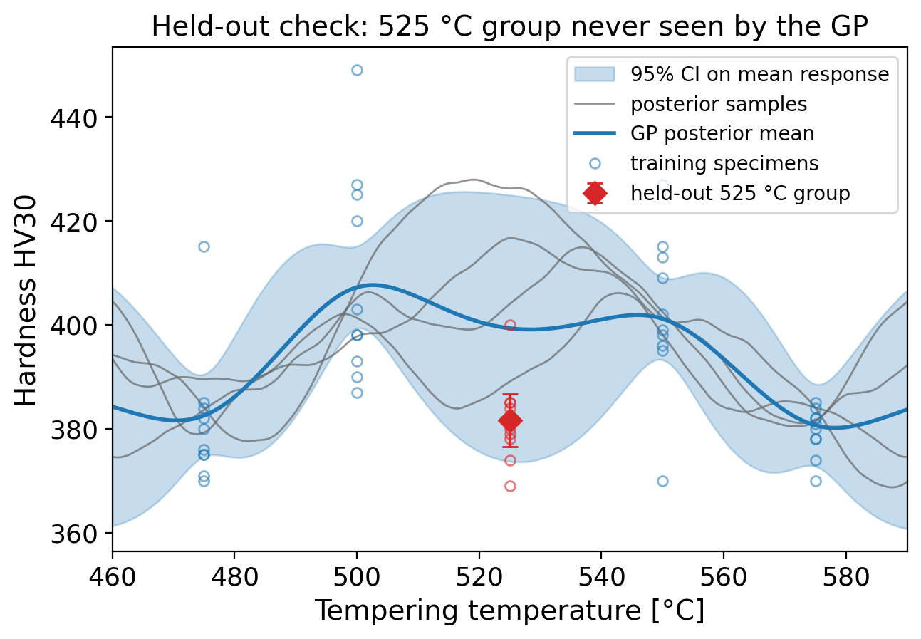
The real test: the 525 °C group (red) was hidden from the GP, which was fit on the other 40 specimens. The held-out group mean lands inside the 95% band.

Note

Trust the ribbon only after a held-out or leave-one-out check says you may — here: 92% empirical coverage for a 95% band.

The shape of the posterior matters more than any single number. Walk the class through the ribbon: tight at sampled points (with 10 replicates the CI on the mean collapses to \(\approx \pm 2\sigma_n/\sqrt{10} \approx \pm 8\) HV30), wide mid-gap (\(\pm 19\) HV30 — the prior takes over), reverting toward \(\sigma_f\) outside the data (next slide). That ribbon shape is the whole reason we used a GP.

Leave-one-out CV is the GP’s free diagnostic. Because the GP posterior is closed-form, leave-one-out predictions are cheap (Sundararajan-Keerthi trick: no refit per fold; our script brute-force refits because \(n = 50\) costs milliseconds). On this fit: 46/50 specimens inside the 95% predictive band — 92% empirical vs 95% nominal, i.e. the band is honest to within the resolution 50 points can check (\(\pm\) a few points is expected binomial fluctuation).

Why the held-out-group check is the one to show. Held-out specimens mostly test the noise model; a held-out condition tests interpolation — the thing we actually want the GP for. The GP fit without the 525 °C group predicts \(399 \pm 26\) HV30; measured \(382 \pm 5\). Two readings: (a) covered — the CI is honest; (b) the point prediction pulled up toward the neighbouring peaks and missed by 17 HV30, and the wide band told you not to trust the point estimate. Both readings are the lesson. If your process decision needs \(\pm 10\) HV30 at an unsampled temper, the GP’s answer is “measure it” — and it says so quantitatively.

Anti-pattern. Reporting \(\pm 1\sigma\) instead of \(\pm 2\sigma\). Always quote 95 % CI (\(\pm 2\sigma\) under Gaussian); \(\pm 1\sigma\) is the standard error, half as wide, and reads like overconfidence to a lab manager.

War story. I once had a student report 90 % CI as “the model says HRC is between 38 and 40”. Two specimens fell at 36 and 41 — exactly the 10 % expected to land outside a 90 % CI. The model was right; the student’s framing made it look wrong. Always communicate CI with the coverage explicitly: “about 1 in 20 specimens will fall outside this band, by construction”.

Cross-reference. §6 reliability diagrams.

Pacing. ~2 minutes.

11. When to trust extrapolation — and when not to

• The GP variance grows back toward \(\sigma_f^2\) as we move away from data.
• For the 1.7709 data: the ribbon balloons outside \([475, 575]\) °C — the model is honestly saying “I have not seen tempers below 475 or above 575, my prediction here is essentially the prior.”
• And the prior mean (391 HV30, the data average) is physically wrong out there: below 475 °C the real response climbs toward the as-quenched \(42 \pm 2\) HRC; above 575 °C tempering-back sets in. The wide band is the only honest part of the extrapolation.

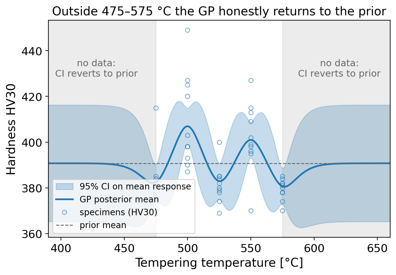
The actual fit, extended beyond the data: inside 475–575 °C the band tracks the measurements; outside, it reverts to the prior within a couple of length scales — the honest answer.

• This is the right answer. Do not clip the variance, do not force-fit a parametric extrapolation. If you need predictions at 625 °C, run the experiment

Warning

The CI growth is only honest if the kernel is correct. A too-long \(\ell\) will make the GP overconfident outside the data. Always cross-check with a held-out CV reliability diagram before you trust extrapolation.

This is the GP’s superpower and the slide students remember. Most surrogate models lie quietly outside their training range: a polynomial fit will extrapolate confidently and wrongly; an MLP will extrapolate confidently and wrongly. The GP says, structurally, “I have not seen this — my prediction is the prior”. That is a feature, not a bug.

The honesty caveat is critical. If you let \(\ell\) optimise too freely and it lands at a too-long length scale (because your data covers a flat region), the GP will think the response is slowly varying and will extrapolate confidently. The fix is a prior on \(\ell\) (informative-prior MAP rather than free MLE), or a Matérn 5/2 with its sharper roll-off. Without those, “honest extrapolation” is a slogan, not a guarantee.

Materials hook. Note what the GP reverts to: the prior mean, here the grand data average (391 HV30). Below 475 °C that is physically wrong — the response climbs toward the as-quenched \(42 \pm 2\) HRC (the paper reports 40–44 HRC after quench, i.e. 392–434 HV) as carbide precipitation slows. The GP does not know this; the wide band is it admitting so. If you have that physics intuition, encode it: a parametric tempering-law mean function (with the GP correcting deviations) would extrapolate downward sensibly and keep honest variance growth. With \(\ell = 13\) °C the reversion happens within ~2 length scales — 25-30 °C past the last data point the model is already back at the prior. Short length scale = short memory; that is the price of resolving the peaks.

Anti-pattern. “Forcing” a parametric extrapolation by fitting a polynomial to the GP’s mean curve and extending it. This loses the honest CI growth — you have replaced a Bayesian model with a deterministic one outside the training range. If you need predictions out there, run the experiment or use a physics model.

Pre-empt. “Could I use a periodic kernel? The fitted curve looks oscillatory.” — good eye, and no: the two peaks come from distinct precipitation reactions (Cr-, then Mo/V-rich carbides), not from a periodic mechanism. A periodic kernel would hallucinate more peaks outside the data with high confidence — the exact opposite of honest extrapolation. Periodic kernels belong where physics is genuinely periodic (cyclic loading, rotating-disc spectra).

Cross-reference. §6 OOD detection — the same “out of training distribution” question, formalised. ML-PC u12 (PINNs) uses physics to extrapolate where data fails.

Pacing. ~1.5 minutes.

12. What this enables — direct ROI

• Pre-GP workflow: 6 destructive tensile + hardness tests per heat treatment recipe, 4 recipes, 24 tests at €200/test → €4 800.
• Post-GP workflow: 3 anchor tests + GP interpolation. CI verified, sufficient for spec compliance on standard heats. 12 tests, €2 400.

• Saved per heat-treatment campaign: ~€2 400. Across a year of campaigns: into the tens of thousands.
• Cost of the GP: half a day of analyst time, no infrastructure.

Warning

Caveat: the GP does not replace verification at the spec extremes. It replaces redundant tests in the smooth interior of the process window.

The ROI slide is for the lab manager, not the student. Students will compute their own ROI for their MSc projects after this slide. Make the numbers concrete: €200/test is a realistic standalone hardness + tensile test in a contract lab; €300 is a printed cube + cross-section + measurement; €1k+/h is analytical S/TEM with operator and amortised tool cost. These numbers are the currency of materials ML.

The half-day analyst cost is real. A working GP fit with kernel selection, hyperparameter optimisation, LOO reliability, and a written-up CI takes a competent analyst roughly half a day — including writing the model card. That is the true cost-to-deploy. Do not let students quote “5 lines of scikit-learn” as the cost; the discipline around the 5 lines is the work.

The spec-extreme caveat matters. A GP cannot replace verification at the spec boundary — that is where the cost of being wrong is highest and where the GP’s CI is most likely to be wrong (boundary regimes, fewer replicates, possible regime changes). Use the GP to skip tests in the interior of the safe region, not at the cliffs.

Scaling up the ROI. One heat-treatment campaign saves €2 400. A medium-sized lab runs 20-50 such campaigns per year. The headline number is €50-100k of test-cost savings annually, against a half-day-per-campaign analyst cost. That is the slide students photograph and send to their advisors.

Anti-pattern. Trying to extend the ROI argument to all tests. The GP saves the redundant interior tests; the spec-edge tests are required for certification. Reframing them as “interpolation” is how you ship a scrapped batch.

Pacing. ~1 minute. Move fast — this is the punchline, not the lecture.

13. Modern small-tabular alternative: TabPFN

• TabPFN (Hollmann et al. 2025) is a transformer pre-trained on millions of synthetic tabular tasks to do in-context prediction — no per-task fitting.
• Pass your 50 rows + new query → it returns a calibrated posterior predictive in one forward pass.
• 2025 version (v2) handles up to \(\sim 10\,000\) rows and is competitive with tuned XGBoost on small-tabular benchmarks.
• Code: github.com/PriorLabs/TabPFN — pip install tabpfn, scikit-learn-compatible API.

When the GP still wins:

• 1-D smooth process variable + interpretable hyperparameters (length scale = physical correlation length).
• You need the posterior closed-form for downstream optimisation (BO acquisition functions, gradient w.r.t. inputs).
• You need to encode prior physics (Matérn smoothness, periodic kernels for cycling processes).

Note

On a 50-row task like the 21CrMoV5-7 data, expect TabPFN and a disciplined GP to give comparable held-out error; the GP wins on interpretability of \(\ell\) and \(\sigma_f\) and on encoding the replicate-based \(\sigma_n\). Use whichever your stakeholder will sign off on — try it as a homework exercise against data_mantzoukas2021_table3.csv.

Why this slide exists in 2026. Until \(\sim 2023\), “small tabular + uncertainty” was synonymous with “Gaussian process.” TabPFN inverts that default for problems where the input space is more than 1-D and where kernel engineering would otherwise dominate the analyst’s day. The transformer is doing implicit kernel learning — billions of synthetic priors absorbed into the weights at pre-training time.

One sentence definition. TabPFN is a frozen Bayesian non-parametric regressor / classifier whose prior was learned (not hand-specified) by pre-training on synthetic data. You query it like a function; it returns calibrated probabilities.

Materials-relevant strengths. (1) In-context — no hyperparameter optimisation per dataset. (2) Calibration out of the box; the posterior is already a probability, not a softmax. (3) Handles mixed continuous/categorical features without one-hot tricks. (4) Inference is \(\mathcal{O}(n^2)\) in the in-context set but the constant is small; \(n = 1000\) runs in seconds on a single 1080Ti.

Materials-relevant limitations. (1) No kernel ⇒ no physical interpretation of length scale or smoothness — black-box prior. (2) Cannot extrapolate honestly outside the pre-training prior — the model has its own implicit OOD failure mode, which is harder to diagnose than a GP’s variance growth. (3) Heavy dependency to install (\(\sim 1\) GB checkpoint).

Connection to MFML W7 (the “Watch for: TabPFN” fragment). That slide introduces TabPFN as the first credible deep-learning approach to small tabular problems. This slide is the materials-specific deployment view.

Anti-pattern. Using TabPFN on \(n > 10\,000\) rows. Above that, gradient-boosted trees beat it and run faster. Stay in TabPFN’s sweet spot.

Forward link. §6 audits calibration with reliability diagrams; TabPFN’s calibrated posterior already gives close-to-honest intervals on in-distribution data — still verify on a held-out lab set.

§D · Case study B — MC Dropout for SEM defect segmentation

14. Setup: U-Net on SEM micrographs

• Task: per-pixel segmentation of SEM micrographs of an additively manufactured steel into {matrix, austenite, martensite/austenite, precipitate, defect} — the public MetalDAM set (ArcelorMittal and DaSCI Andalusian Research Institute 2021; Luengo et al. 2022).
• Architecture: U-Net with dropout layers (\(p \approx 0.2\)) in the bottleneck and decoder.
• Training data: 42 expert-segmented micrographs \(\to\) \(\mathcal{O}(10^3)\) 256×256 tiles; whole micrographs held out for evaluation. The second tool (“SEM #2”) is simulated below by a detector gamma/contrast/noise shift — MetalDAM is single-source.

• The point estimate (argmax over softmax) is fine on the training distribution and bad on the deployment distribution. We need a per-pixel uncertainty map to flag the bad regions.

• Hands-on: reproduce this entire case study in the Week-13 notebook — Colab-ready, data via ai4mat.datasets.MetalDAMDataset.

Warning

Always evaluate on a session or tool you did not train on — a random split of one SEM session hides exactly the drift that breaks deployment.

Why segmentation, why MC Dropout. Segmentation is the one task where you want UQ per pixel, not per image. A 1024×1024 SEM tile is ~1M decisions; even a 99 % per-pixel accuracy means ~10 000 wrong pixels per tile — enough to lose the small pores that matter most. MC Dropout gives you a spatial uncertainty map for the same training cost as a deterministic U-Net. That is a deal you cannot easily refuse.

The data is real; the tool shift is simulated. All §D figures come from an actual run (make_mcdropout_figures.py, seed 0) on MetalDAM — 42 SEM micrographs of AM steel from ArcelorMittal with expert pixel labels; class shares are heavily imbalanced (austenite 58%, matrix 32%, M/A 9%, defect 0.7%, precipitate 0.2%). MetalDAM comes from a single instrument, so the “SEM #2” evaluation applies a physically motivated detector perturbation (gamma 0.75, contrast ×1.3, brightness +0.04, extra noise σ=0.02) to the held-out micrographs — say this out loud; on your own data you should always evaluate on a tool you did not train on. (For a multi-category SEM benchmark without pixel masks, see Modarres et al. (Modarres et al. 2017) — classification only, which is why it is not used here.)

Dropout placement matters. Dropout in the bottleneck + decoder is the standard recommendation: too early and the early features collapse; too late and the variance is tiny because you have already committed to a class. \(p \approx 0.2\) is the typical sweet spot; below 0.1 the variance collapses (the well-known MC-Dropout pathology in deep modern networks); above 0.4 training stalls.

Anti-pattern. Adding dropout only at training time and forgetting to keep it on at inference. PyTorch’s model.eval() switches dropout off — you have to call enable_dropout() or use model.train() to keep it stochastic. About half of student MC-Dropout implementations get this wrong silently.

Cross-reference. ML-PC u04 (CNNs / U-Net) for the architecture; ML-PC u06 (DINOv2 transfer) for the alternative — pretrained features + light head. MFML W12 for the variational-Bayes interpretation.

Pacing. ~1.5 minutes.

15. MC Dropout in practice

• Training: standard, dropout active.
• Inference: keep dropout on, run \(T = 30\) stochastic forward passes per image.
• Per pixel \(i\): collect \(\{p_i^{(t)}\}_{t=1}^{T}\) — softmax distributions over classes.
• Predictive mean: \(\bar{p}_i = \tfrac{1}{T}\sum_t p_i^{(t)}\) → argmax for the class label.
• Per-pixel predictive entropy: \(H_i = -\sum_c \bar{p}_{i,c} \log \bar{p}_{i,c}\) — the uncertainty map.

Note

\(T{=}30\) is the typical knee — below 10 the variance estimate is too noisy, above 50 you are paying for diminishing returns. Validate \(T\) on a held-out reliability diagram.

Two quantities, two stories. - Predictive mean \(\bar p_i\) → the prediction. Use argmax of \(\bar p\), not of any single pass — averaging removes the dropout noise. This is consistently 0.5-2 IoU points better than a single deterministic forward. - Predictive entropy \(H_i\) → the uncertainty. High \(H\) either means several classes are competing (epistemic) or the predicted class is near-uniform (aleatoric on a hard boundary). For UQ purposes we treat the entropy as a single uncertainty score; separating aleatoric from epistemic requires mutual information (see Depeweg et al. 2018) and is rarely worth the complexity.

The \(T=30\) heuristic. Why 30? Variance of a Monte Carlo mean scales as \(1/T\); the variance of the variance estimator scales as \(1/T\) too, so doubling \(T\) from 30 to 60 only tightens the variance estimate by \(\sqrt 2\). Below \(T=10\) you cannot tell calibrated from broken; above \(T=50\) you pay linearly with no payoff. Tell students to measure the knee on their own task with a reliability diagram, not to trust 30 blindly.

Compute budget (measured). \(T=30\) on a 256×256 tile took 0.07 s on an RTX A6000 in our run (make_mcdropout_figures.py); on a 1080Ti-class workstation card expect roughly 1–2 s per tile. Fine for offline analysis (tens of tiles/day on a benchtop SEM), too slow for inline detection at 1 Hz on modest hardware. If real-time, drop to ensembles (parallelisable) or temperature-scaled deterministic + Mahalanobis OOD.

Anti-pattern. Using the variance of softmax outputs instead of the entropy of the mean softmax. They are different quantities and have different calibration properties; the predictive-entropy of \(\bar p\) is what the variational interpretation calls “total uncertainty”.

Cross-reference. Gal & Ghahramani (2016) is the seminal paper; the materials extension is straightforward. MFML W12 for the variational-approximation derivation.

Pacing. ~3 minutes — the formulas slide.

16. Per-pixel uncertainty maps — what they look like

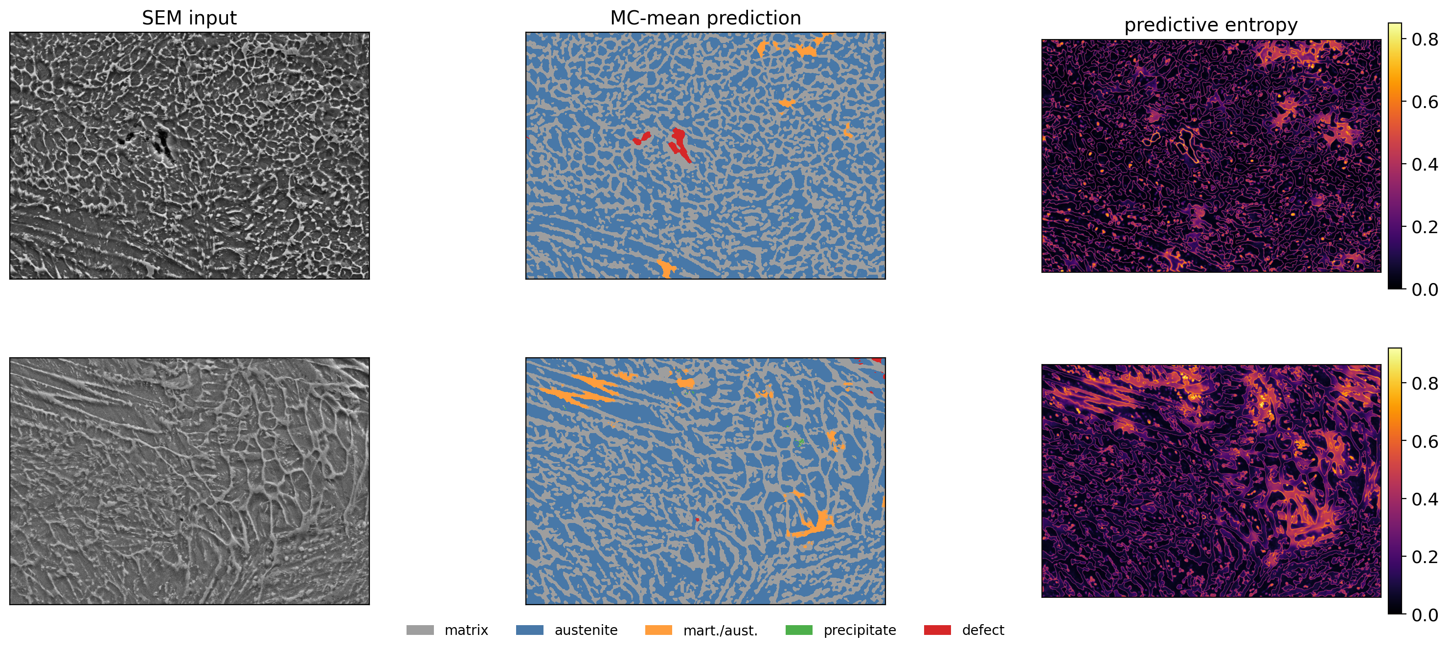
Two held-out MetalDAM micrographs: SEM input, MC-mean prediction, per-pixel predictive entropy (\(T{=}30\)). Low entropy inside well-formed austenite/matrix regions; high entropy at phase boundaries, inside ambiguous martensite/austenite laths, and at defect rims.

Note

These are diagnostic: the model is honestly uncertain exactly where a human operator would also hesitate. On your own instrument, FoV/tile edges and charging halos light up the same way.

The slide where MC Dropout earns its keep. A well-calibrated uncertainty map is self-interpretable: the high-entropy regions overlap exactly with where you, the human expert, would zoom in and look harder. If your map does not have that property, you have a calibration bug (most likely dropout too low, or only one dropout layer).

Demo opportunity. If you have a teaching SEM micrograph with a known charging halo (insulator next to conductor), show the entropy map next to the input image. Charging zones light up. Students gasp. This is the slide that converts the skeptics.

What the figure actually shows (our MetalDAM run). High entropy concentrates (i) on austenite/matrix phase boundaries, (ii) inside martensite/austenite regions — the class the annotators themselves find hardest, IoU 0.43 — and (iii) at defect rims. Precipitates are essentially unlearnable in MetalDAM (IoU ~0.01) because most were left unannotated (stated in the dataset README) — a live example of the u03 label-noise lecture.

The generic failure modes to name beyond this figure. - Grain-boundary triple junctions: legitimate class ambiguity; the model is right to hesitate. - FoV edges: receptive-field artefact; cropping fix or boundary-aware loss. - Charging zones: physical SEM artefact; the model is correctly refusing — pass it to a human or to a charge-compensation preprocessor. (MetalDAM has no charging halos; show one from your own instrument if available.) - Tile edges: stitching artefact; overlap-and-blend at inference.

Anti-pattern. Smoothing the uncertainty map (Gaussian blur) before thresholding. Spatial resolution of the entropy map is its point; smoothing destroys the diagnostic value. If the map is too noisy, increase \(T\) or fix the dropout placement.

Cross-reference. ML-PC u09 (segmentation in spectroscopy) uses the same diagnostic pattern. MFML W12 for the formal “the model is honest about what it does not know” claim.

Pacing. ~2 minutes.

17. Reject-for-human-review threshold

• Pick a per-pixel entropy threshold \(\tau\). Pixels with \(H_i > \tau\) are flagged for operator review; the rest are auto-classified.

• Sweep \(\tau\) to draw the operating curve: (human-review rate) on the x-axis vs (defect recall) on the y-axis.
• The threshold is a business decision, not an ML decision — it depends on the cost of a missed defect vs the cost of operator time.

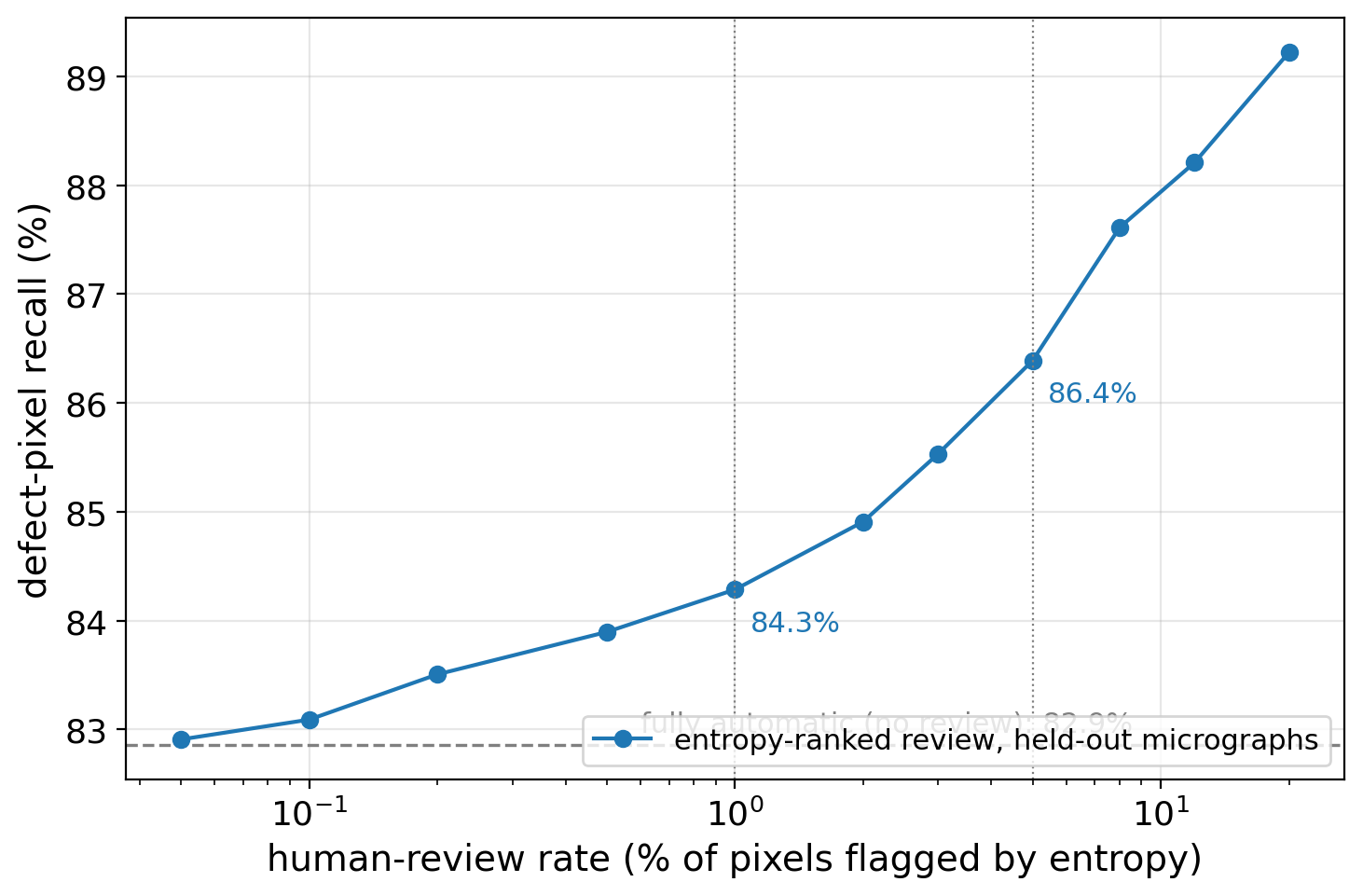
Measured on the held-out MetalDAM micrographs: fully automatic recovers 82.9% of defect pixels; entropy-ranked review adds +1.4 points at 1% review and +3.5 points at 5%. The residual misses are low-entropy — confidently wrong — pixels, which no amount of entropy-ranked review recovers: exactly why the calibration audit on the next slide matters.

Note

Report the operating curve, not a single threshold — the deployment context picks the operating point.

This is a real engineering decision. Make sure students understand: the threshold is not “set by the ML method”; it is set by operational cost. Two labs running the same model will pick different thresholds based on what their analyst hour costs and what a missed defect costs.

The operating-curve mindset. Treat this like an ROC curve: the model gives you a sliding tradeoff, and the deployment context picks the operating point. “86 % recall at 5 % review” is one point on the curve; the curve itself is the deliverable. Always plot it.

Numerical interpretation (our run). Auto-only recall is already 82.9% because the weighted loss makes the model defect-sensitive; entropy-ranked review then buys +1.4 points at 1% review and +3.5 at 5% (89.2% at an unrealistic 20%). There is no sharp knee here, and the gap to 100% is the honest headline: the remaining defect pixels are confidently wrong — the entropy map cannot flag them, only recalibration (next slide) or more labels can. At 5% review on a 1024×703 micrograph that is ~36k flagged pixels — clusterable into a few hundred ROIs an analyst scans in under a minute.

Anti-pattern. Reporting only a single threshold (“we used \(\tau = 0.5\)”). The threshold has no meaning without the operating curve. If the paper does not show the curve, the operating point is unjustified.

Cross-reference. This pattern (model + human review) is exactly the human-in-the-loop active learning setting we get back to in §5 — uncertain pixels become the next labelled tiles.

Pre-empt. “Should I use Bayes risk minimisation instead?” — yes, when you can quantify the costs explicitly. In most lab settings, costs are not known (intangibles like reputation, certification risk), so a curve + business-side choice is more honest than a single optimisation.

Pacing. ~2 minutes.

18. Tool-shift calibration

• The reliability diagram on SEM #1 (training tool) is well-calibrated.
• The reliability diagram on SEM #2 (different detector, different bias) is not — the model is overconfident on a slightly different contrast distribution.

• Practical fix: per-tool temperature scaling. Collect a small (~50 image) calibration set on the new tool, fit a single scalar \(T\) to recalibrate. Cheap, post-hoc, no retraining.
• Re-run calibration after any: detector swap, gun replacement, sample-coating change, large chamber vent.

Note

“My segmentation accuracy dropped after the chamber vent” is a calibration failure as often as a model failure. Diagnose with a reliability diagram before retraining.

The single most underrated slide in the deck. Most students who deploy a model and watch performance drop will immediately assume retraining is the fix. Wrong first move: run the calibration audit (\(\sim 50\) images, 5 minutes of work) before touching the weights. Be precise about what recalibration buys — our run shows both sides: temperature scaling restored honest confidences (ECE 9.2% → 3.5%), so every confidence-thresholded downstream step (reject-for-review, defect triage) works again, but it cannot restore raw pixel accuracy (argmax is unchanged; 59% stays 59%). If the accuracy loss itself is unacceptable, that is a fine-tuning decision — made after the audit, not instead of it.

Why a single scalar \(T\) works. Temperature scaling (Guo et al. 2017) divides logits by \(T\) before softmax: \(\hat p = \text{softmax}(z/T)\). It is a one-parameter rescaling that does not change argmax — the predictions stay the same, only the confidences change. So retraining the entire network is not required when only the confidence calibration has drifted. This is the slide that gets a “huh” reaction from the audience.

When recalibration is not enough. If the argmax predictions themselves are wrong on the new tool (true distribution shift, not just calibration drift), temperature scaling cannot rescue you. The diagnostic: predicted-class accuracy at low temperature (i.e., where the model is forced to commit). If that drops, you need fine-tuning or a new model.

The trigger list is real. Detector swaps, gun replacements, coating changes, large chamber vents — each one shifts the contrast distribution enough to break a softmax calibration. Re-run the reliability diagram on day 1 of any of these events.

War story. A collaborator’s pore-detection pipeline (segmentation + confidence-thresholded defect triage) dropped from 96 % to 78 % end-to-end after a routine chamber clean. They retrained for two weeks and recovered to 91 %. The actual bug: the contrast shift had broken the calibration, so the fixed confidence threshold silently discarded most true detections — temperature scaling on 30 calibration images restored the thresholding step in an hour. (Note the mechanism: recalibration can rescue a confidence-thresholded pipeline; it never changes the raw argmax accuracy.) The training time was wasted; the diagnosis was the bug.

Cross-reference. §6 reliability diagrams (the diagnostic); ML-PC u02 (physics-of-data; the chamber vent is a physics-of-the-instrument issue).

Pacing. ~3 minutes — this is the slide where most students update their mental model of “deployment”.

§E · Case study C — Active learning loop for AM process windows

19. Setup: laser powder-bed fusion process map

• Process: laser powder-bed fusion (L-PBF) of 316L stainless steel, fixed layer thickness (30 µm) and hatch spacing (120 µm).
• Two-axis design space: laser power \(P \in [125, 350]\) W and scan speed \(v \in [100, 3400]\) mm/s — the ranges of the 35-cube dataset of Diaz Vallejo et al. (2021) that grounds this case study.
• Goal: identify the process window — the region in \((P, v)\) where relative density \(\rho_{\text{rel}} > 0.995\): below it, keyhole porosity (low \(v\)); above it, lack-of-fusion porosity (high \(v\)).

• Each experiment: print a \(\sim 5\) mm cube, cross-section, measure \(\rho_{\text{rel}}\) — about €300 in materials, machine time, and metallography.

Note

Every point in the \((P, v)\) plane costs €300 — the experiment budget, not the model, is the scarce resource.

Why L-PBF is the canonical AM-AL case study. Two continuous inputs (power, speed), one measurable scalar output (relative density), explicit safety constraints (keyhole regime damages the optics), and a real per-experiment cost (€300/cube including operator + metallography). It has every feature you need to teach AL, with no time-series or multi-physics distractions.

The physical landscape. The \((P, v)\) plane has a “process window” bounded by: (a) low energy density → lack-of-fusion porosity; (b) high energy density → keyhole porosity + melt-pool collapse; (c) extreme \(P/v\) → instability and spatter. The shape of the window depends on the alloy and the layer thickness; it is not a rectangle. AL is the right tool because the window’s boundary is what we want to find, and the boundary is geometrically nontrivial.

Why €300/experiment is realistic. Materials (~€20 of powder), machine time (~€100, 30 min on a benchtop), cross-section + mount + polish + image analysis (~€150, half an analyst-day). Industrial systems are higher.

Anti-pattern. Starting AL on a process you do not understand at all. AL is exploitation-biased — if your initial surrogate is badly mis-specified, AL will spend the budget exploring the wrong region. Always seed with 5-8 grid-style points to cover the design space before switching to AL.

Cross-reference. Hernández-Lobato_2014_PES in ref.bib for the foundational Bayesian-optimisation-for-materials paper; ML-PC u14 (reflection) for the broader self-driving-lab framing.

Pacing. ~2 minutes. The setup is concrete; spend the time on the loop slide next.

20. The active-learning loop

• GP surrogate: \(\rho_{\text{rel}}(P, v)\) with a 2-D RBF or Matérn kernel, separate length scales \(\ell_P, \ell_v\).
• Acquisition function:
  • Upper Confidence Bound: \(\alpha_{\text{UCB}}(P,v) = \mu(P,v) + \beta\,\sigma(P,v)\).
  • Expected Improvement: \(\alpha_{\text{EI}}\) favours points likely to beat the current best.
• Choose the next experiment to maximize \(\alpha\) — trade off mean (exploitation) vs variance (exploration) (Hernández-Lobato et al. 2014).

Note

Honest \(\sigma\) is what makes the exploration–exploitation trade fair — a miscalibrated surrogate sends the €300 experiments to the wrong place.

The closed-loop diagram is the conceptual heart of self-driving labs. Every Materials Acceleration Platform (MAP) — Berlinguette’s “Ada”, Aspuru-Guzik’s “ChemOS”, Mooney’s photonics loop — is exactly this picture with a different surrogate and a different instrument. Once students see this loop, they see every modern AM-+-ML paper through it.

Why UCB and EI, and when each wins. - UCB (\(\mu + \beta\sigma\)): explicit knob \(\beta\) to control exploration. Easy to tune, easy to explain to non-ML collaborators, no normality assumption. Default for new loops. - EI: integrates over the probability of improvement, weighted by how much improvement. More expensive to evaluate (no closed form for non-Gaussian posteriors), but better when the goal is finding the optimum, not mapping the window. - For “find the process window” (this case study), I usually start with UCB because the boundary is the deliverable, not the maximum density.

Length scales matter. Separate \(\ell_P\) and \(\ell_v\) are essential — power and speed have different physical effects on the melt pool. ARD (automatic relevance determination) is built into most GP libraries; turn it on.

Anti-pattern. Running AL on a deterministic simulator-derived “data” set with no real measurement noise. AL then converges in 5 iterations to the simulator’s optimum, which is not the real-world optimum. AL only earns its keep when the experiments are real.

Pre-empt. “Why not Bayesian Neural Networks instead of a GP surrogate?” — at \(n < 100\), the GP wins on calibration and on closed-form acquisition gradients. Switch to BNNs / ensembles only when \(n\) outgrows the GP’s \(O(N^3)\) ceiling.

Cross-reference. Hernandez-Lobato_2014_PES (foundational AL/BO paper); MFML W12 for the closed-form acquisition gradients.

Pacing. ~3 minutes. This is the slide students photograph.

21. Closed loop with the printer + safety constraints

• Hard constraints the acquisition cannot violate:
  • \(P/v\) ratio — prevent keyhole regime that damages optics.
  • Absolute caps — machine specs.
  • “No-go” zones from prior failures — flagged manually.

• Constrained Bayesian optimization: \(\max_{(P,v)} \alpha(P,v)\) subject to \(g_k(P,v) \leq 0\).
• Implementation: rejection sampling on the candidate set, or a second GP modeling the constraint probability.
• Budget cap: stop the loop after \(N_{\max} = 30\) experiments or when the process-window area stabilizes — whichever comes first.

Warning

Safety constraints must be hard constraints — a soft penalty that “usually” avoids the keyhole regime will eventually damage the optics.

Safety constraints turn BO into constrained BO. In a research demo you do unconstrained BO and call it done. On a real printer you have hard constraints: keyhole damages the laser optics; absolute power/speed limits are machine spec; the no-go list grows after every failed print. Constrained BO is the only acceptable version in a lab. Make this explicit.

Two implementations, two trade-offs. - Rejection sampling on the candidate set is trivial and cheap when the constraint is a known closed-form (e.g., \(P/v < 1\) J/mm). Use this when you have a physics-derived constraint. - Constraint-GP models the probability the constraint holds, learned from past experiments. Use this when constraints are discovered empirically (e.g., “this specific (P,v) caused melt-pool collapse last Wednesday”). Combine with EI to get constrained EI.

The budget cap is operationally important. AL without a stopping rule runs until you cancel it; that is the wrong default for a shared printer. Two stopping rules in tandem: (a) hit \(N_{\max}\) (budget); (b) the area of high-density region stops growing for 3-5 consecutive iterations (convergence). When either triggers, stop. Tell students this before they run their first loop and waste a weekend’s powder budget.

War story. I once had an AL loop run unattended over a weekend. The keyhole constraint was missing from the candidate-set filter. Monday morning: damaged optics on the printer, ~€8 000 to repair, and one analyst in a very bad mood. The constraint was the first thing we added on Tuesday. Always test the constraint logic before running unattended.

Anti-pattern. “Soft” constraints (penalties added to the acquisition function). For safety constraints you want a hard constraint — the acquisition cannot propose a keyhole condition, ever. Penalties allow occasional violations and that is unacceptable.

Cross-reference. Constrained-BO references in ref.bib; ML-PC u14 (reflection) for the broader self-driving-lab framing.

Pacing. ~2.5 minutes.

22. Visualizing AL vs Grid: How does active learning discover the process window?

• Plot: x-axis = number of experiments; y-axis = area of process window confidently classified (\(P[\rho_{\text{rel}} > 0.995] > 0.9\)).
• Mechanism: AL curve rises steeply — acquisition functions (UCB / EI / straddle) steer experiments straight to the window boundary.
• Grid-search baseline: \(14 \times 14 = 196\) experiments to cover the design at matching resolution; AL requires far fewer.

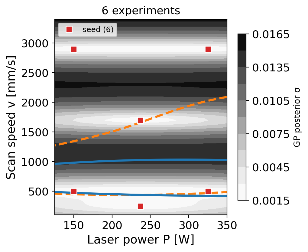
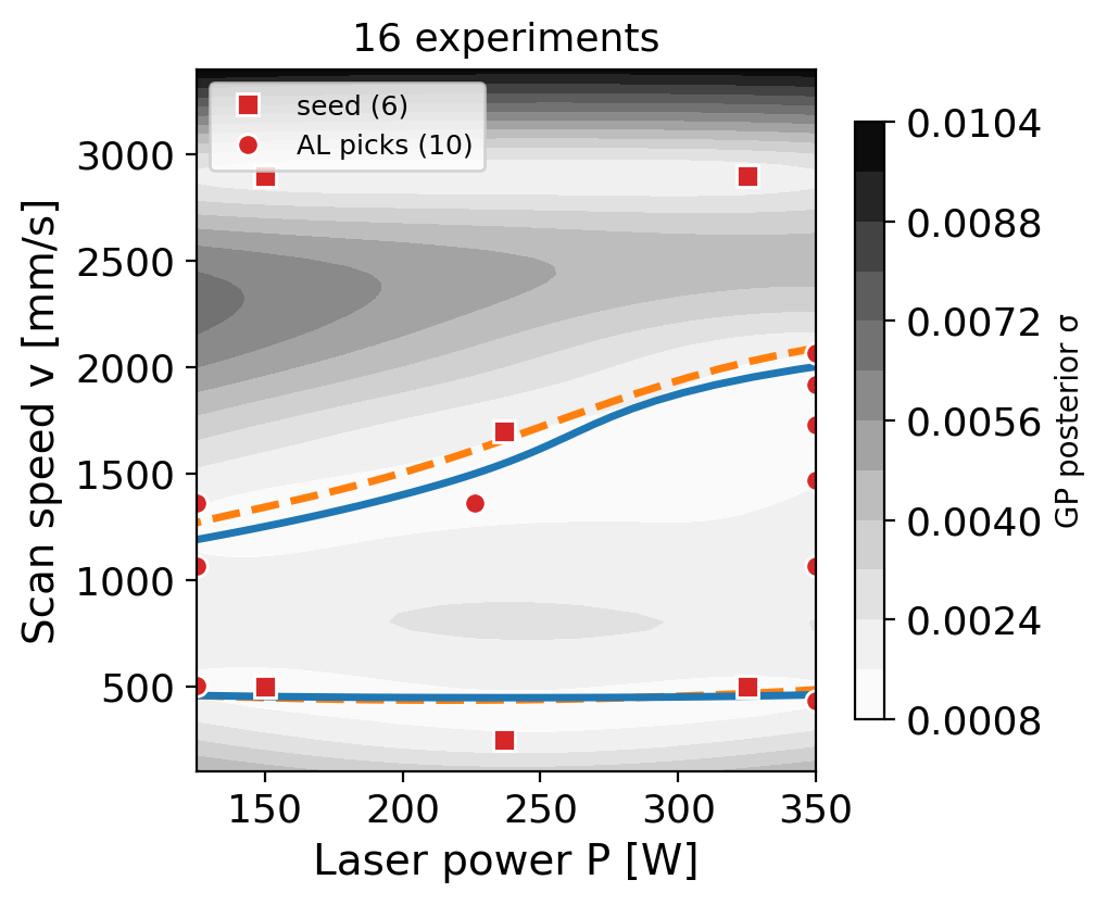
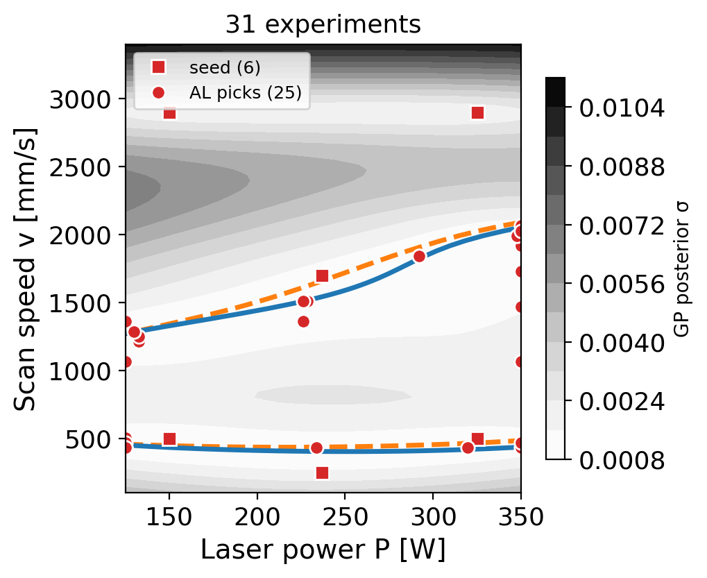
Seed design only (6 cubes): GP \(\sigma\) (grey) high everywhere; the estimated \(\rho_{\text{rel}}{=}0.995\) boundary (blue) is far from the true one (orange, dashed) — 20% misclassified.

After 10 picks (16 exp): AL routes every cube to the boundary — misclassification drops to 2.7%.

After 25 picks (31 exp): Both window boundaries are sharply localized; grid at this res = 196.

Note

Active learning beats grid search — the actual lab default, not just random sampling.

What the images show: Actual AL run on surface fit to the Diaz-Vallejo 316L dataset (\(\sigma=0.002\) noise), not synthetic data. GP with straddle acquisition focuses sampling on the process window’s boundary (where it’s hardest and most valuable). 6 seeds → 16 → 31 experiments, and the process window is quickly localized; grid would need 196. Simulated campaign — mechanism, not the result, is key: AL clusters effort where the boundary is sharpest.

Steep early gain: UCB/EI/straddle focus cubes right where high uncertainty (variance) meets high value: the edge of the process window. The interior fills in last.

23. AL Efficiency: Headline numbers & cost savings

• Campaign results (8 seeds): 31 AL cubes confidently identify 83% ± 5% of the true window; a \(9 \times 9 = 81\)-cube grid is needed to match.
  ⇒ ~2.6× reduction in experimental cost.
• Budget impact: At €300/experiment: €15,000 saved per material.
  And, savings increase further in higher dimensions (add hatch, preheat…).

• Why not just dense sampling (grid or Latin hypercube) + GP fit?
  That gives a map — but not a sharp boundary.
  AL is built to find boundaries by sampling where uncertainty is highest.

Note

The real benchmark is grid search, not random sampling. AL outperforms the common lab practice and accelerates discovery.

Measured, not quoted: Real campaign, real numbers: 8 random seeds; average 31 AL cubes = 83% window found; grid needs 81. AL consistently gets more window for fewer experiments. At typical lab cost, this is €15k per alloy, and effects multiply in higher input dimensions.

Framing for students: Grid-search is still what most labs do by default (“let’s sweep a grid”). AL gives a path to accelerate discovery, save resources, and shrink timelines — especially as the parameter space grows. Plot headline numbers up front, then explain why AL’s focusing behavior makes this possible.

23. The effort curve — AL vs grid, 8 random campaigns

• \(y\)-axis: fraction of the true window area confidently identified — \(P[\rho_{\text{rel}} > 0.995] > 0.9\) and actually inside the window.
• Shaded bands: \(\pm 1\) std over 8 random campaigns (jittered seed designs + fresh measurement noise) — single-seed AL curves are not evidence.

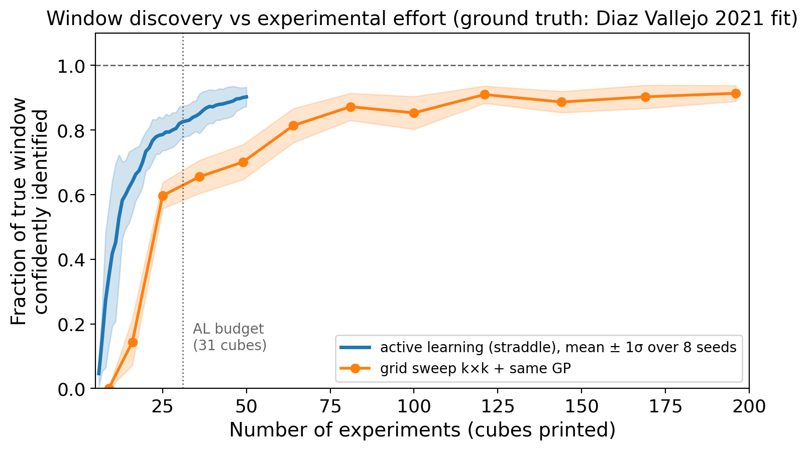
Active learning (blue) vs \(k{\times}k\) grid sweep + the same GP (orange), both on the Diaz-Vallejo-grounded surface. AL reaches 83% of the window at 31 cubes; the grid needs 81 to match. Both saturate near ~90%: the last sliver of window hugs the boundary, where \(P > 0.9\) classification would require replicate cubes.

Note

The AL advantage is the steep early slope — under a hard experiment budget you stop exactly in the regime where AL is far ahead of the grid.

How to read the figure. Same ground truth, same GP, same noise — the only difference between the curves is which cube gets printed next. The straddle acquisition spends every cube on the level set; the grid spends most cubes in the interior and the corners where the classification is already easy or hopeless.

The honest numbers. AL at 31 cubes: 82.6% ± 4.9% of the true window confidently identified. The grid needs 9×9 = 81 cubes to reach that level. That is a ~2.6× cost reduction in this 2-D, 316L-grounded campaign — real, but not the 6-7× sometimes quoted. Two reasons: (a) in 2-D a grid is a respectable design; the AL advantage grows with input dimension (add hatch spacing, layer thickness, preheat…); (b) both curves saturate near 90% because the remaining window area hugs the boundary, where confident classification at σ = 0.002 needs replicates, not more single cubes.

Why the bands matter. This is the anti-pattern from the previous slide done right: 8 campaigns with jittered seed designs and fresh noise. The AL band (± 5%) is the honest statement of run-to-run variability; a single lucky seed can look 10 points better.

Pre-empt. “Why does the grid curve wobble downward at some sizes?” — coarse grids can straddle the boundary luckily or unluckily; the GP’s confident region shifts with where the grid points happen to land relative to the level set.

Pacing. ~2 minutes. Read the two numbers off the plot, state the two saturation reasons, move on.

24. Materials-acceleration-platform framing

• This loop — surrogate model + acquisition + closed-loop instrument + safety constraints — is the prototype of a self-driving lab.
• Aspuru-Guzik and Berlinguette groups have built versions of this loop for catalysis and thin-film electrochemistry. Same pattern, different instrument (Hernández-Lobato et al. 2014).

• The only ingredient that makes this work is honest UQ. With overconfident or miscalibrated \(\sigma\), the acquisition function picks the wrong next experiment and you waste your budget. UQ is not a slide at the end — it is the engine.

Warning

With a miscalibrated \(\sigma\) the loop still runs — it just spends your budget on the wrong experiments, and nothing in the loop’s output tells you.

The framing slide. This is where students realise the entire unit so far has been about MAPs. The §3 GP teaches the surrogate; §4 MC-Dropout teaches per-pixel UQ for instrument-screen; §5 AL closes the loop with an instrument. MAPs are the deployment context.

The Aspuru-Guzik / Berlinguette / NIMS lineage. Multiple research groups have built versions of this loop for catalysis (Ada, Berlinguette), drug discovery (ChemOS, Aspuru-Guzik), thin films (NIMS Japan, USTC China), polymers (BASF), and increasingly metals (CMU, NIST). The loop is not a research toy any more — Toyota, BASF, and several US national labs run versions of it in production. Tell students this is the standard of 2026, not the frontier of 2018.

Why honest UQ is the engine, restated. If \(\sigma\) is overconfident → AL converges prematurely and misses regions. If \(\sigma\) is underconfident → AL never commits and wastes budget. If \(\sigma\) is miscalibrated heterogeneously → AL is biased toward the falsely-confident region. None of these are detectable from the loop’s outputs; all of them are detectable from a held-out reliability diagram before you start the loop. Calibrate first, then run.

Anti-pattern. Treating AL as “set and forget”. Real MAPs have a human in the loop — a researcher who looks at the next-proposed experiment, sanity-checks it, and approves or vetoes. The day you remove that human is the day you damage the instrument (see the keyhole war story).

Cross-reference. ML-PC u14 (reflection on the course) returns to MAPs as the future of materials research. This is the slide that bridges to it.

Forward link. §6 is the next slide — calibration as the engine of every MAP.

Pacing. ~2 minutes. Big-picture, not technical.

§F · Calibration & deployment hygiene

25. Reliability diagrams on lab data

• Bin predictions into 10 confidence bins. For each bin, compare predicted confidence vs observed accuracy (or coverage of the CI).
• Perfect calibration: diagonal.
• Above the diagonal: under-confident. Below: over-confident (the dangerous failure mode).

• Where typical materials models break:
  • Out-of-distribution alloy family — model is highly confident, accuracy collapses.
  • Different microscope / coating / operator — softmax stays at 0.95+, accuracy drops 20 points.
  • Long-tail rare defect classes — confidence is high on the wrong class.

Warning

Always run a reliability diagram on a held-out, lab-realistic calibration set — not a random split of the training data.

The diagnostic plot of the whole unit. A reliability diagram is not optional — it is the single piece of evidence that converts a model from “fits well on test set” to “trustworthy for deployment”. If a paper, thesis, or model card lacks one, the UQ claims are unsubstantiated.

How to read the diagram in 30 seconds. Bin predicted confidences into 10 bins (0-10 %, 10-20 %, …). For each bin, plot empirical accuracy (y) vs mean predicted confidence (x). Diagonal = perfectly calibrated. Above diagonal = the model is less confident than it should be (under-confident — annoying but safe). Below diagonal = over-confident — the dangerous mode, the one that ships scrap.

The three named failure modes are the materials ones. - Alloy family shift: composition outside training distribution; softmax stays high, predictions wrong. - Microscope/coating/operator shift: pixel statistics differ; softmax stays high, predictions wrong. - Long-tail rare classes: model memorised “matrix” 95 % of the time, never saw the rare crack class enough; high confidence on the wrong class because the wrong class is the prior.

The lab-realistic calibration set is the key word. A random 80/20 split of the training data is not lab-realistic — it has the same distribution as training. The correct calibration set is prospectively collected on a different day, ideally a different instrument, ideally by a different operator. The point of the calibration set is to mimic the deployment shift. Skipping this is the single most common UQ mistake in published materials-ML.

Anti-pattern. Reporting Expected Calibration Error (ECE) without showing the diagram. ECE is a one-number summary of the diagram; the shape of the curve (is it consistent over-confidence? bin-specific? bimodal?) carries the diagnosis. Always show the picture.

Pre-empt. “Why not just temperature-scale once and call it done?” — temperature scaling fixes miscalibration (vertical scaling of confidence) but cannot fix distribution shift (the model is making wrong argmax predictions, not just wrong confidence). The reliability diagram tells you which one you have.

Cross-reference. Guo et al. 2017 (the original temp-scaling paper); MFML W12 for the formal definition of calibration; ML-PC u04 (CNN training) for cross-validation discipline.

Pacing. ~3 minutes.

26. OOD detection — when the model sees something new

• Symptoms: confidence is high, prediction is wrong. Calibration alone cannot save you — you need to detect the OOD case and refuse to predict.

• Workflow: train your model, fit a Mahalanobis detector on training features, reject any inference with detector score above a threshold and route to a human.

Practical detectors:

• Mahalanobis distance in feature space (penultimate-layer activations vs the training-set Gaussian) — cheap, surprisingly effective on microscopy.
• Ensemble disagreement — for a deep ensemble, high prediction variance across members \(\Rightarrow\) OOD. Free if you already have an ensemble.
• GP variance — for GP surrogates, \(\sigma^2 \to \sigma_f^2\) flags inputs far from training. This is the same mechanism as the AL loop in §E.

Note

Calibration and OOD detection are separate responsibilities — a perfectly calibrated model still needs a detector that refuses to predict off-distribution.

Calibration ≠ OOD detection. This is the slide that splits two ideas students conflate. Calibration says “given an in-distribution input, my \(p\) matches my accuracy”. OOD detection says “this input does not look like training, refuse to predict”. Both are mandatory; neither subsumes the other.

Mahalanobis is the workhorse. Why it works: penultimate-layer activations of a CNN trained on natural-ish images are approximately Gaussian. Fit a multivariate Gaussian (one per class) on the training features; at test time, compute the minimum-class Mahalanobis distance. High distance ⇒ OOD ⇒ refuse. Cheap, training-free post-hoc, and the materials-ML literature consistently finds it competitive with much more elaborate detectors.

Ensemble disagreement. If you have an ensemble (§2), the variance across members is an OOD signal — high variance on a new image suggests members disagree because they have not seen it. Free if the ensemble exists; expensive if you have to train one for OOD detection alone.

GP variance is the textbook example. \(\sigma^2 \to \sigma_f^2\) outside training data — by construction. The §3 GP and the §5 AL loop both use exactly this property. The GP is the one model where calibration + OOD are the same mechanism.

Workflow detail not on slide. Setting the OOD threshold: take a held-out lab-realistic OOD set (e.g., images from a different microscope you definitely did not train on), compute Mahalanobis distance on training-distribution and OOD-distribution images, pick the threshold at the desired false-positive rate (e.g., reject 1 % of in-distribution to catch 95 % of OOD). Same operating-curve logic as §4’s reject-for-review.

Anti-pattern. Using softmax entropy as an OOD signal. Modern overconfident networks have low entropy even on OOD inputs — the softmax is not the right detector. The Mahalanobis distance lives in feature space, which is much better.

Cross-reference. Lee et al. 2018 (Mahalanobis OOD detector); Liu et al. 2020 (energy score). ML-PC u06 (transfer learning) is where OOD is most acute.

Pacing. ~3 minutes.

27. Reproducibility hygiene

• Random seed logged for: data split, model init, dropout sampling, ensemble members, BO acquisition.
• Model card alongside the model artifact: training data version, test metrics, calibration plot, OOD detector ROC, list of known failure modes.
• Dataset version pin: hash of the labeled set; never silently update.

The one-paragraph “uncertainty section” of a model card:

“Uncertainty is reported as 95% CIs from \(T{=}30\) MC-dropout passes. The model is calibrated by temperature scaling on a 200-image held-out set; expected calibration error 0.03. The model is in-distribution iff Mahalanobis score \(<\tau_{\text{OOD}} = 14.2\); outside that, predictions are not returned.”

Note

If you cannot write that paragraph for your model, you cannot deploy it.

The “deployment checklist” slide. This is the closing-discipline slide of the unit. If a student remembers only one slide from §6, this should be it: the things you have to log to claim you have shipped a trustworthy model.

Random seeds matter for UQ specifically. Calibration and AL results change with seed. Logging the seeds (data split, model init, dropout, ensemble, BO acquisition) lets you reproduce. Not logging them is the cheapest mistake in materials-ML deployments — papers regularly fail to replicate because of unlogged seed.

Model cards. Hugging Face popularised the term; in materials we adapt it: training data version + hash, test metrics, calibration plot, OOD detector ROC, list of known failure modes (with named examples — “fails on uncoated insulating samples”, “fails on alloy family X”, “fails after chamber vent”). One markdown file shipped with every model artifact. Tell students to write this before deploying, not after.

Dataset version pin matters more than you think. Labelled materials data sets are quietly updated all the time — a labeller corrects a few mistakes, the dataset becomes “labels v1.1”. Without a hash pin, the model you trained is no longer reproducible six months later. Always pin the hash; treat the dataset like code.

The one-paragraph uncertainty section is the deliverable. Read it aloud, slowly. Every clause is necessary. “Uncertainty is reported as 95 % CIs from \(T=30\) MC dropout passes” (method + parameter); “calibrated by temperature scaling on a 200-image held-out set” (calibration evidence); “ECE 0.03” (number); “Mahalanobis OOD detector with threshold 14.2” (OOD policy). If your model card lacks any of these, the model is not deployable.

Anti-pattern. “We will write the model card after the paper is accepted.” No — the model card is the thing that earns the acceptance. Skip it and the model is undeployable, regardless of how well the paper reads.

Cross-reference. Mitchell et al. 2019 (the model cards paper); ML-PC u14 (reflection — model cards as the unit of accountability in materials ML).

Pacing. ~2 minutes. Read the paragraph, make students notice every clause.

28. What MFML covers that we skipped

Pointer slide. If you want the math behind today’s tools:

MFML W12 (uncertainty in predictions):

• Bayesian predictive distribution and the variance decomposition (aleatory + epistemic).
• Marginal likelihood / evidence framework as automatic Occam’s razor.
• Closed-form GP posterior (mean + variance), kernel hyperparameter learning by log marginal likelihood.
• ELBO and variational interpretation of MC Dropout.
• Calibration formalism (reliability, ECE) and recalibration methods (temperature scaling, Platt, isotonic).

MFML W8 (tree ensembles & tabular):

• TabPFN’s prior-data fitted network — what the pre-training prior actually is.

• In ML-PC: we use these results on real lab data. Pick the right tool, validate it on a reliability diagram, and trust the answer enough to skip a destructive test or pick the next experiment.

Note

Read the MFML math first, then deploy with this deck open — the reverse order produces copy-pasted snippets with no diagnostic intuition.

The bridge slide. This is the slide that defines the relationship between the two courses for students taking both. ML-PC is the applied sibling of MFML; today’s unit consumes MFML W12 the way an engineering course consumes a thermodynamics course. Tell students this aloud.

For the MFML attendees. Their next-week lecture in MFML W12 is the math behind everything we used today. They should walk into MFML W12 with the practical motivation from this unit fresh in their heads — that improves retention dramatically. Active pre-loading.

For the ML-PC-only attendees. They do not need to re-derive the math to deploy these tools, but they do need to know which assumptions matter. The bullet list on this slide is also the “things to look up in Bishop / Murphy if a deployment surprises you” list.

Anti-pattern. Trying to learn the math during deployment. The right order is: read MFML W12, then deploy with the today’s deck open. Reverse order leads to copy-pasted scikit-learn snippets with no diagnostic intuition.

Cross-reference. MFML W12 (Bayesian inference deep dive). Bishop ch.3 and ch.6 are the standard textbook treatment.

Pacing. ~1 minute. This is a pointer, not a re-lecture.

§G · Wrap

29. Recap: Unit 12

1. Pick the UQ tool per task: GP or TabPFN for small tabular data, MC dropout for trained CNNs, ensembles for high-stakes regression, MDN for multi-modal outputs.
2. Calibrate before deploying — a reliability diagram on a held-out lab-realistic set is non-negotiable.
3. UQ enables active learning — and active learning is how labs scale beyond the brute-force grid search.
4. OOD detection complements calibration — confidence is meaningless when the input is outside the training distribution.
5. The math lives in MFML W12 (Bayes, GP, calibration). ML-PC W13 is about using that math to save tests, find process windows, and ship trustworthy models.

Note

A model without calibrated uncertainty fails silently; a model with it tells you exactly which experiment to run next.

The five-line takeaway. Each of the five items in the recap maps onto a specific section of the deck: 1. Tool-per-task → §2 (decision table) + §3-4 (case studies). 2. Calibrate first → §6 reliability diagrams; the single most important deployment-side message. 3. UQ enables AL → §5 (AM process windows); UQ is the engine, not the ornament. 4. OOD detection → §6 Mahalanobis; calibration and OOD are separate responsibilities. 5. The math is in MFML W12 → bridge to the sibling course.

Closing line for the lecture. “A model without honest, calibrated uncertainty is a deliverable that fails on Tuesday and you do not know why. A model with it is a deliverable that fails on Tuesday and tells you exactly which experiment to run to fix it. That distinction is the whole subfield.”

Exam hint without saying “exam”. If the exam contains an open-ended question about deployment, the rubric is this slide. Tool choice + calibration + AL + OOD + math pointer = full marks. Tell them.

What the homework will ask. Take the §3 GP example, run it on your own tabular data set, produce a leave-one-out reliability diagram, write the model-card uncertainty paragraph. That homework is the practical test of whether the unit landed.

Back link. Unit 11 (PINNs, the previous deck) showed how to bring physics into the model itself — replacing parts of the data-driven prior with a hard physics prior. UQ + PINNs together is the modern frontier.

Pacing. ~3 minutes for the recap + closing line. Then take questions.

Continue

• ← Previous: Unit 11 — Physics-informed and constrained ML
• → Next: Unit 13 — Integration, limits, and reflection
• All courses

30. References & further reading

• Mantzoukas et al. (2021) — 21CrMoV5-7 quench-and-temper data used in §C (Mantzoukas et al. 2021).
• Modarres et al. (2017) — SEM benchmark for the segmentation/classification setup of §D (Modarres et al. 2017).
• Diaz Vallejo et al. (2021) — 316L L-PBF process-parameter/density dataset grounding the §E active-learning campaign (Diaz Vallejo et al. 2021).
• Gal & Ghahramani (2016) — MC Dropout as approximate Bayesian inference (Gal and Ghahramani 2016).
• Lakshminarayanan et al. (2017) — Deep ensembles, the empirical gold standard for NN UQ (Lakshminarayanan et al. 2017).
• Hernández-Lobato et al. (2014) — Predictive entropy search; foundational for BO/active learning in materials (Hernández-Lobato et al. 2014).
• Guo et al. (2017) — Modern NNs are miscalibrated; temperature scaling (Guo et al. 2017).
• Hollmann et al. (2025) — TabPFN v2, foundation model for tabular data (Hollmann et al. 2025).
• Rasmussen & Williams (2006) — GP reference text.
• Aspuru-Guzik & Berlinguette — self-driving lab perspective; materials-acceleration platforms.
• MFML W12 — full mathematical treatment of all methods used here.

ArcelorMittal, and DaSCI Andalusian Research Institute. 2021. MetalDAM: Metallography Dataset from Additive Manufacturing. https://github.com/ari-dasci/OD-MetalDAM.

Diaz Vallejo, N., C. Lucas, N. Ayers, K. Graydon, H. Hyer, and Y. Sohn. 2021. “Process Optimization and Microstructure Analysis to Understand Laser Powder Bed Fusion of 316L Stainless Steel.” Metals 11 (5): 832. https://doi.org/10.3390/met11050832.

Gal, Yarin, and Zoubin Ghahramani. 2016. “Dropout as a Bayesian Approximation: Representing Model Uncertainty in Deep Learning.” International Conference on Machine Learning, 1050–59. https://proceedings.mlr.press/v48/gal16.pdf.

Guo, Chuan, Geoff Pleiss, Yu Sun, and Kilian Q. Weinberger. 2017. “On Calibration of Modern Neural Networks.” International Conference on Machine Learning, 1321–30.

Hernández-Lobato, José Miguel, Matthew W. Hoffman, and Zoubin Ghahramani. 2014. “Predictive Entropy Search for Efficient Global Optimization of Black-Box Functions.” Advances in Neural Information Processing Systems 27.

Hollmann, Noah, Samuel Müller, Lennart Purucker, et al. 2025. “Accurate Predictions on Small Data with a Tabular Foundation Model.” Nature 637: 319–26. https://doi.org/10.1038/s41586-024-08328-6.

Lakshminarayanan, Balaji, Alexander Pritzel, and Charles Blundell. 2017. “Simple and Scalable Predictive Uncertainty Estimation Using Deep Ensembles.” Advances in Neural Information Processing Systems 30. https://papers.nips.cc/paper_files/paper/2017/hash/9ef2ed4b7fd2c810847ffa5fa85bce38-Abstract.html.

Luengo, Julián, Raúl Moreno, Iván Sevillano, et al. 2022. “A Tutorial on the Segmentation of Metallographic Images: Taxonomy, New MetalDAM Dataset, Deep Learning-Based Ensemble Model, Experimental Analysis and Challenges.” Information Fusion 78: 232–53. https://doi.org/10.1016/j.inffus.2021.09.018.

Mantzoukas, John, Dimitris G. Papageorgiou, Carmen Medrea, and Constantinos Stergiou. 2021. “Hardness Behavior of W. Nr. 1.7709 Steel, Oil Quenched and Tempered Between 475–575 c.” MATEC Web of Conferences 349: 02005. https://doi.org/10.1051/matecconf/202134902005.

Modarres, Mohammad Hadi, Rossella Aversa, Stefano Cozzini, Regina Ciancio, Angelo Leto, and Giuseppe Piero Brandino. 2017. “Neural Network for Nanoscience Scanning Electron Microscope Image Recognition.” Scientific Reports 7: 13282. https://doi.org/10.1038/s41598-017-13565-z.