ECLIPSE Presentations – Data Science for Electron Microscopy Week 7: Beating small & expensive data

Recap: Week 6 and today’s question

Week 6: CNNs for microscopy — convolution as a sliding detector, weight sharing, feature hierarchy, U-Net for pixel-accurate segmentation.
Core insight: a pretrained CNN is a hierarchical feature extractor — Layer 1 detects edges, deeper layers detect grain boundaries, phases, defects.
The uncomfortable reality: to train a reliable CNN you typically need hundreds of labelled images. One labelled SEM micrograph of an additive-manufactured alloy can take hours of sample preparation plus another hour of expert annotation — one labelled image.
Today’s question: you have 30 labelled TEM frames. How do you train a model that actually generalises?
Answer: three complementary strategies — data augmentation, transfer learning, and synthetic data — combined into one workflow.

Open by asking who noticed the Week 6 forward-link bullet: “training a U-Net from scratch on EM data requires 50–200 annotated images; transfer learning can reduce this to 20–50.” Today delivers that promise.
The one point to land: the three strategies are not alternatives — they are used together. A real EM pipeline might start with Voronoi synthetic data, augment extensively, and fine-tune from an ImageNet-pretrained backbone.
Misconception to preempt: “if CNNs need so many labels, they are useless for EM.” Wrong. The techniques today make them feasible with 20–50 carefully chosen labels.
EM anchor: make the cost concrete. Ti-6Al-4V SEM cross-section: half a day of sectioning, mounting, grinding, polishing, etching; another hour of expert grain segmentation. That is one labelled image. Compare to ImageNet where a crowdworker labels “dog” in two seconds.
Pacing: 3 minutes maximum. The conceptual slides start on the next slide.
Transition: “Let me show the roadmap and then the concrete data-cost numbers.”

Road map and self-study

Road map: recap Week 6 + today’s question (2) · the small/expensive-data reality in materials (5) · data augmentation: core idea; physical invariances; geometric; intensity; invalid augmentations; on-the-fly; laser-weld scenario; Albumentations code (8) · transfer learning: why features transfer; ImageNet→EM; domain gap; backbone and head; decision matrix; recipe freeze→head→fine-tune; catastrophic forgetting; gradual unfreezing (7) · synthetic data and digital twins: free labels; Voronoi pipeline; why it transfers (3) · the sim-to-real gap; domain adaptation; Voronoi limits; failure scenario (4) · active learning (2) · cross-material transfer (1) · putting it together: complete workflow; published evidence; validation; checklist; quantitative summary; Voronoi→SEM pipeline (6) · forward link to Week 8 (1).
Self-study: notebooks/week07_transfer_finetune.ipynb — pretrain a tiny CNN on abundant synthetic “task A” (Voronoi-like), then compare (i) from-scratch on few task-B labels vs (ii) transfer (freeze backbone, train head); plot loss and accuracy curves; vary label count and observe the transfer gap shrink. All CPU-fast on tiny data. Slide numbers in this deck match the notebook section headers.

The labelled-data gap: a three-order-of-magnitude problem

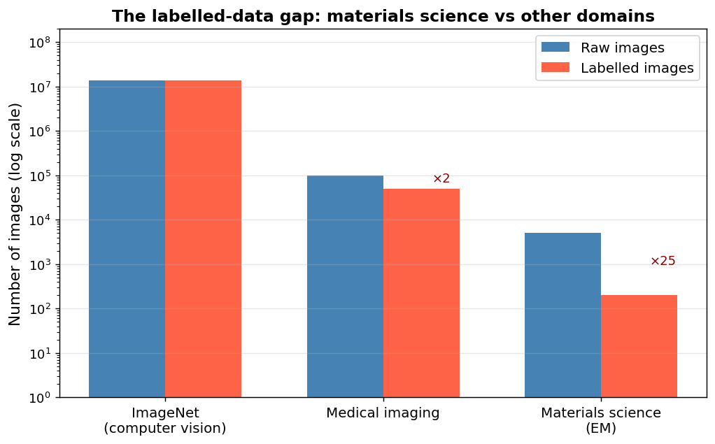
Labelled image counts across domains. ImageNet: 14 million images, crowdsourced labels in seconds. Medical imaging: tens of thousands, expert radiologists. Materials science / EM: 50–500 images, PhD microscopists spending hours per image Holm, Elizabeth A. et al., (2020); Sandfeld, Stefan et al., (2024). Three orders of magnitude separate us from where standard deep learning was designed to work.

Walk through the three bars. The key number: materials science sits three orders of magnitude below where ResNet-50 (25 million parameters) was designed to operate.
The one point to land: the bottleneck is not pixels — a 4D-STEM dataset is hundreds of GB of raw frames. The bottleneck is expert annotation time. Raw data is abundant; labelled data is scarce.
Misconception to preempt: “materials labs have terabytes of data, so data is not scarce.” Separate raw data from labelled data. A 4D-STEM scan has millions of diffraction patterns, none of which come with a label until a human expert provides it.
EM anchor: name two specific costs. (1) Prior-β grain segmentation in titanium: half a day sample preparation + one hour expert annotation = one labelled image. (2) EELS chemical-state labelling of a defect map: requires comparing to reference spectra, knowledge of oxidation states, judgment about beam-damage artefacts — hours per image.
Transition: “The consequence for a naive deep learning approach is catastrophic — overfitting.”

Why labels cost so much in EM

High acquisition cost: synchrotron beamtime, aberration-corrected TEMs costing €3–8 M — access is rationed.
Expert annotation time: segmenting 100 grains in an SEM image takes hours; identifying defect types in an HAADF image requires crystallography expertise and literature comparison.
Reproducibility barriers: a Zeiss and a FEI SEM of the same specimen produce systematically different contrast — pooling raw images from two instruments silently introduces a domain shift that corrupts a naive model.
Limited specimen availability: a cross-section of a real additively-manufactured turbine component may be unique — you cannot re-image or re-annotate.
The rule of thumb: in materials EM, expect 50–500 labelled images for a typical task. ResNet-50 has 25 million parameters — at 500 images that is 50 000 parameters per image. Guaranteed overfitting without outside help.

Overfitting in the small-data regime: the mechanism

Overfitting = the model memorises the training set rather than learning generalisable patterns.
With 50 labelled images, a ResNet-50 (25 M parameters) has ~500 000 parameters per training image. There are enough degrees of freedom to perfectly fit any labelling of those 50 images — including the noise.
Typical EM overfitting shortcuts (what the model actually memorises):
- Detector vignetting: images acquired with the same gain settings at the same session are brighter at the centre. The model learns “bright centre → class A” rather than “class A microstructure.”
- Scale bar position or font: if images from one class systematically had the scale bar in one corner, the model learns the corner, not the microstructure.
- Microscope/operator session: instrument-specific contrast baseline, beam-damage patterns, contamination level.
The diagnostic: run Grad-CAM (gradient-weighted class activation map). If saliency lights up on the image corner, the scale bar, or the vignette — not on the microstructure — you have a shortcut model.

Small data → fast overfitting

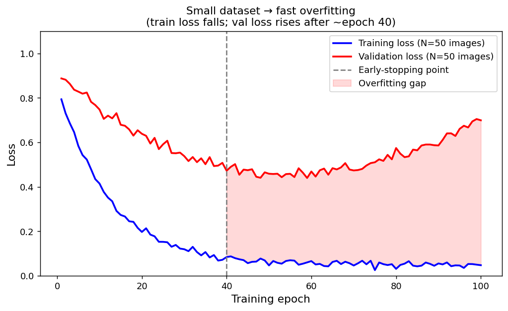
Training and validation loss for a CNN fine-tuned from scratch on 50 EM images. Training loss falls monotonically; validation loss starts rising around epoch 40 — the model is memorising the training images, not learning to generalise. The gap is the overfitting region.

Walk through the two curves. “Training loss falls nicely — the model can memorise 50 images in 40 epochs. Validation loss follows for a while, then diverges: the model is fitting per-image noise — detector vignetting, brightness drift, instrument-specific contrast — not physical microstructure.”
The one point to land: the typical EM failure mode is not “the model is wrong” on training data — it is 100% training accuracy and 55% test accuracy (barely better than chance for a binary task). The symptom is the train-val gap, not training loss.
Misconception to preempt: “I can fix overfitting by training longer.” No. Training longer makes overfitting worse. The fixes are: more labelled data, augmentation, transfer learning, or synthetic pre-training. All three are today’s topic.
EM anchor: a published war story: a weld-defect classifier hit 99% training / 58% test. Grad-CAM revealed the model had learned the SEM vignetting pattern (brighter at centre) that happened to correlate with the imaging session for good welds. Fix: brightness augmentation + grouped cross-validation.
Transition: “Three strategies attack this problem. Let me introduce them together.”

The small-data survival kit: three strategies

Strategy 1 — Data augmentation: apply physically plausible image transformations to multiply the effective training set size. Forces the network to learn invariant features, not per-image artefacts.
Strategy 2 — Transfer learning: start from a CNN pre-trained on ImageNet (1.4 million images). The first layers’ edge and texture detectors transfer to EM images — we only need to adapt the last layers.
Strategy 3 — Synthetic data: generate Voronoi microstructures (or physics simulations) and get perfect ground-truth labels at zero annotation cost. Pre-train on thousands of synthetic images; fine-tune on the 30 real ones.
Critical rule: these three strategies are not alternatives — they are orthogonal levers used together. The production answer is: synthetic pre-training → augmentation throughout → ImageNet or synthetic backbone → fine-tune on real labelled data.

Augmentation: the core idea

What augmentation does: take one labelled image and apply a transformation → produce a new image that looks different but represents the same physical content with the same label.
What this achieves: the network must produce the same prediction for the original and the transformed versions. Any features that change under the transformation become uninformative. The model is forced toward invariant (physics-faithful) features.
Concrete example: applying a horizontal flip forces the boundary detector to fire regardless of which side of the image the boundary is on — encoding the physical fact that grain boundaries look the same everywhere.
On-the-fly is preferred: sample a fresh random transform every epoch. 50 images × 8 random transforms per epoch × 100 epochs → the network sees ~40 000 distinct views. Offline augmentation (pre-generate on disk) produces a fixed set the network will eventually memorise.

Augmentation: encoding physical invariances

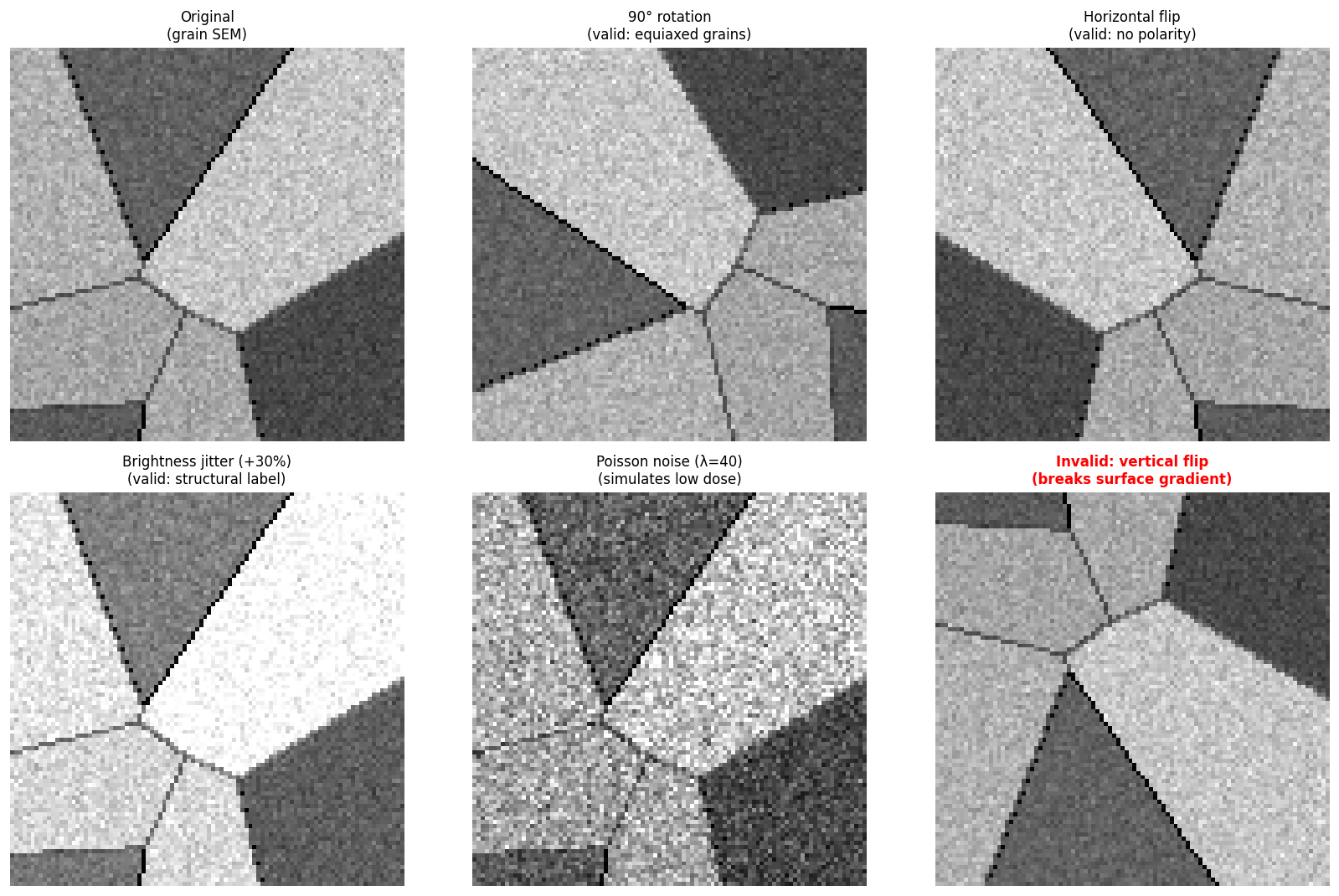
Six augmented views of the SAME synthetic grain microstructure. All six panels show the same Voronoi grain layout (same polygonal grains, same topology) transformed in different ways. Top row: original, 90° rotation (valid for equiaxed grains), horizontal flip (valid — no polarity). Bottom row: brightness jitter (valid — structural label), Poisson noise (simulates low dose), vertical flip (invalid — breaks a surface gradient if present). Each valid transform is a claim that the physics has a symmetry.

The key concept for this slide: augmentation is not just multiplying data — it encodes a claim that the physics has a particular invariance. A rotation augmentation says “a grain boundary looks the same at any angle.” That is true for equiaxed grains; it is false for directionally solidified columnar grains, where orientation is a physical signal.
The one point to land: “before adding any transform, ask: would this produce a physically plausible image with the same label? If not, it is label noise you injected by hand.”
Misconception to preempt: “more augmentation is always safer.” Wrong. A wrong augmentation actively harms the model by injecting false invariances. Ablate augmentations one at a time if performance is unexpectedly poor.
EM anchor: for equiaxed recrystallised grains, rotation is truly invariant (orientation is arbitrary). For a thermal-gradient zone or rolled-sheet texture, rotation is physically meaningless. Same type of image, opposite correct answer — the difference is the physics.
Transition: “The most important augmentation concept is not the transforms themselves but the legality gate — next slide.”

Geometric augmentations: what they encode

Horizontal / vertical flip: encodes mirror symmetry. Valid for most equiaxed microstructures; invalid if the feature has polarity (e.g. surface-hardening layer — “top” differs from “bottom”).
Rotation (90°, 180°, 270°, or arbitrary): encodes rotational symmetry. Valid for equiaxed grains; invalid for directionally solidified columnar structures or any feature where orientation is the label.
Random crop / zoom: encodes translation and scale invariance. Usually safe, but ensure the crop does not eliminate the feature you are trying to detect.
Elastic deformation: simulates sample warping or electron-beam drift. Valid for topology-based tasks (grain boundary present/absent); invalid if metric properties (grain size, aspect ratio) are the label — elastic warp silently corrupts quantitative ground-truth.
Label consistency rule: every geometric transform applied to the image MUST be applied identically to the mask, bounding box, or label. Rotate image AND mask by the same randomly-sampled angle, at the same time.

The label consistency rule is the most common bug in augmentation pipelines for segmentation. Symptom: training loss looks fine but IoU plateaus — the model is training on systematically misaligned ground truth.
The anti-pattern is calling the transform twice — once on the image, once on the mask — which samples two independent random angles. Use Albumentations: transform(image=img, mask=mask) applies one sampled transform to both jointly. This single API fact is worth knowing.
The one point to land: geometric transforms are claims about physical symmetries. Make the claim explicit; if the physics does not have the symmetry, the augmentation is harmful.
EM anchor: elastic deformation on a grain-size regression task. The deformed image is augmented; the grain area labels now refer to elastically-distorted grains whose true areas are no longer correct. The model learns to regress on corrupted labels. Symptom: lower accuracy on real images than expected from training curves.
Transition: “Intensity transformations are generally safer — but not always.”

Intensity augmentations and noise

Brightness / contrast jitter (±10–20%): makes the model robust to session-to-session detector variation and illumination drift. Valid when the label is structural (grain present/absent, defect class). Invalid when the label is calibrated to absolute intensity (EELS chemical quantification, BSE Z-contrast phase fractions).
Gamma correction: simulates non-linear detector response. Usually valid for structural tasks.
Gaussian noise: simulates electronic readout noise — signal-independent variance. Valid; does not corrupt structural labels.
Poisson (shot) noise: the physically correct noise model for EM — signal-dependent, dominant at low dose. Augmenting with Poisson noise simulates low-dose imaging and is the best insurance against cross-session contrast variation in beam-sensitive experiments.
Blur (Gaussian or motion): simulates defocus or sample drift. Forces the model to rely on topology, not fine texture — exactly the property that makes synthetic grain-boundary detectors transfer to real SEMs.

The Poisson noise point is the materials-literate distinction. Generic CV courses add Gaussian noise. In EM the physically correct noise is Poisson — signal-dependent, worst at low dose, directly related to beam damage constraints. A model augmented with realistic Poisson noise transfers to low-dose acquisition; one trained only on clean images fails when you reduce dose to protect the sample.
The intensity-quantitative exception is important and often missed. Brightness jitter is illegal for EELS/EDS quantification because absolute intensity IS the label (composition fraction). State it explicitly.
The one point to land: intensity augmentations are generally safer than geometric ones, but the physics gate still applies: if the label is intensity-calibrated, intensity transforms corrupt it.
EM anchor: a carbon-contamination detector trained with brightness jitter starts ignoring subtle intensity changes that are the only signal of contamination onset. The augmentation erased the very feature it was meant to detect.
Transition: “Now the materials-specific subtlety that no generic CV course covers: physically-illegal augmentations.”

Physically-invalid augmentations: the materials gate

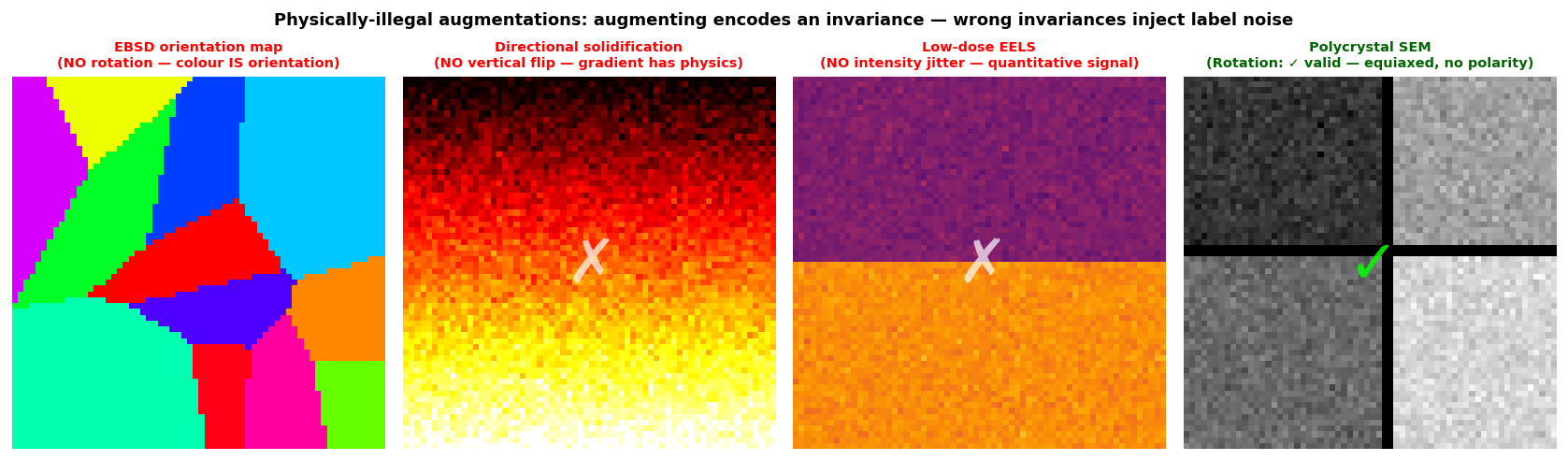
Four panels illustrating when augmentations are illegal. Panel 1 (EBSD map): rotation is illegal — the colour encodes crystallographic orientation; rotating the image without rotating the IPF colour key produces a physically impossible map. Panel 2 (directional solidification): vertical flip is illegal — the thermal gradient is physically real. Panel 3 (EELS map): intensity jitter is illegal — calibrated intensity encodes composition. Panel 4 (equiaxed polycrystal): all augmentations checked here are valid.

This slide is the materials-specific key concept of the augmentation section — spend time here.
The three illegal cases and their precise reasoning:
1. EBSD rotation: the colour in an IPF map IS the crystallographic orientation relative to the sample reference frame. Rotating the image without rotating the colour key produces a pixel that says “orientation 30°” in a location that the crystal assigns “orientation 120°.” It is a labelling error with perfect data fidelity.
2. Directional solidification vertical flip: top of a DS column is the liquidus end (last to solidify), bottom is the solidus end (first). Their microstructures differ (segregation, dendrite morphology). A vertical flip swaps them. The label “grain size at top” now refers to the bottom.
3. EELS jitter: if the label is “this pixel has composition 42% Fe,” and you apply ±20% intensity jitter, the model learns to map the jittered intensity to 42% Fe — which is wrong for the real (non-jittered) measurement.
The one point to land: augmentation legality is a domain-knowledge decision, not a data-science one. Ask a materials scientist, not a CV tutorial.
Misconception to preempt: “these edge cases are rare.” They are not. EBSD, directional solidification, and EELS quantification are three of the most common EM data types. Students will encounter all three.
Transition: “Augmentation is the cheapest lever. The second lever imports knowledge from outside your dataset.”

On-the-fly augmentation and label consistency

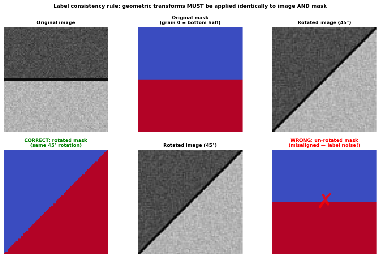
Label consistency: when a grain-boundary image is rotated 45°, the segmentation mask must be rotated by exactly the same 45°. Top row (left to right): original image, original mask, rotated image (45°). Bottom row: correct — rotated mask (same 45°, joint transform); wrong — un-rotated mask paired with the rotated image, producing misaligned ground truth.

On-the-fly (preferred): sample a new random transform per batch — the network never sees exactly the same pixels twice. Near-infinite effective dataset from 50 images.
Offline augmentation: pre-generate augmented images on disk. Faster per epoch but with a fixed set that the network will eventually memorise over many epochs. Use only when augmentation is computationally expensive (e.g. physics rendering).
The rule: augment AFTER splitting by specimen. Augment only the training set. Never augment before the train/test split — an image and its rotation must not land on both sides of the split.

The split-first ordering is the single most common validation error in augmentation pipelines. Name it explicitly: “augmentation leakage” — a rotated copy of a training image ending up in the test set. The test performance then measures memorisation recall, not generalisation.
The practical rule for the exam: SPLIT (by specimen), THEN augment. Never the reverse.
The one point to land: on-the-fly augmentation on 50 images gives near-infinite diversity because the random parameters are resampled each epoch. Offline augmentation on the same 50 images, say 10 variants each, gives 500 frozen images the network will memorise in a few hundred epochs.
EM anchor: five specimens × 10 crops = 50 images. Wrong: split 40 random crops / 10 random crops → every specimen on both sides → the model learns specimen identity. Right: split 3 specimens / 2 specimens → never seen any crop from test specimens. Then augment the 30 training crops to 300+.
Transition: “Augmentation makes the most of data we have. Transfer learning brings in knowledge from outside.”

Augmentation scenario: a laser-welded joint

Scenario: 50 SEM images of a laser-welded joint. The weld bead runs left-to-right. Task: classify weld quality (good/defective).
Apply the physics gate to each proposed augmentation:
- Horizontal flip: Valid — the weld is approximately mirror-symmetric about its centreline; a left-right flip produces a physically plausible weld of the same quality class.
- Vertical flip: Invalid — top surface (cap bead, possible undercut) ≠ root (penetration, possible lack-of-fusion). A vertical flip produces a weld that cannot physically exist.
- 90° rotation: Invalid — the weld runs left-to-right; rotating 90° makes it vertical. Bead direction is physically defined (travel direction, gravity during solidification).
- Brightness jitter: Valid — quality is a structural judgement, not an absolute-intensity measurement; intensity perturbations add robustness to session/detector variation.
- Gaussian noise: Valid — same reason as brightness jitter.
The meta-point: every verdict came from physics, not from a CV default.

Run this as a cold-call question before showing the verdicts. Ask the room: “Horizontal flip — valid or invalid?” Wait for responses. Reveal the verdict AND the physical reasoning.
This scenario is from the source unit and is the canonical worked example for the augmentation legality gate. It makes the abstract principle concrete.
The one point to land: a strong exam answer cites the physical reason, not just the verdict. “Vertical flip is invalid because top surface differs from root” is a passing answer. “Vertical flip is invalid” with no reason is not.
Misconception to surface: “horizontal flip is always safe.” Only here because of the symmetry; it would be wrong for a chiral or single-sided feature. The rule is task-dependent, not image-dependent.
Transition: “The Albumentations code pattern for implementing safe augmentation.”

Augmentation pipeline: Albumentations code

The key API pattern: apply one sampled transform to image AND mask simultaneously — guarantees label consistency for segmentation tasks.

import albumentations as A
transform = A.Compose([
    A.HorizontalFlip(p=0.5),
    A.RandomRotate90(p=0.5),
    A.GaussNoise(var_limit=(10, 50), p=0.3),
    A.RandomBrightnessContrast(p=0.3),
    A.ElasticTransform(alpha=120, sigma=6, p=0.2),
])
result = transform(image=image, mask=mask)  # ONE call, joint transform

transform(image=img, mask=mask) samples one random configuration and applies it to both. The mask and image stay aligned.
The classic bug: calling transform(image=img) and transform(image=mask) separately — two independent random angles — mask and image become desynchronised. Symptom: IoU plateaus with no obvious cause.
Each line is a physics claim: HorizontalFlip claims mirror symmetry; ElasticTransform claims drift robustness; RandomBrightnessContrast claims the label is structural, not intensity-calibrated.

Why ImageNet features transfer to EM images

Transferability as a function of CNN depth Yosinski, Jason et al., (2014). Layer 1 (edges, gradients): ~95% transferable — universal low-level image features. Layer 2 (textures, corners): ~80% — mostly domain-general. Layer 3 (object parts): ~45% — becoming domain-specific. Layer 4+ (full objects / task-specific): ~10% — ImageNet-dog features are not EM features.

This is the theoretical anchor for all of transfer learning. The depth-wise picture is Yosinski et al. 2014. State it as a principle rather than a specific citation: “transferability decreases monotonically with depth.”
Why this is true: early layers are constrained by the statistics of natural images (edges, 1/f spectra, local correlations). EM images share those statistics — they are images, they have edges, they have textures. Late layers are optimised for the specific 1000 ImageNet categories (dogs, chairs, cars) — these have no counterpart in grain boundaries or atomic columns.
The actionable consequence: fine-tuning strategy should be depth-graded. Keep early layers nearly fixed (tiny LR), adapt late layers more (higher LR), and fully retrain the head. This is differential LRs and gradual unfreezing, both of which come on the next slides.
Misconception to preempt: “ImageNet has no TEM images — how can it possibly help?” Early layers learn edge and texture detectors, not dog features. Those edge detectors fire at grain boundaries exactly the same way they fire at the boundary of a dog’s ear. The transfer is at the level of the visual front-end, not the semantic content.
EM anchor: a grain boundary is detected by a “structured region vs unstructured region” contrast — exactly what ImageNet’s first convolutional layers are superb at. They did not need to see gold nanoparticles during training; they needed to see contrast changes, which are universal.
Transition: “The recipe for using this is: backbone plus head.”

The domain gap: ImageNet vs EM images

Natural images (ImageNet): 3-channel 8-bit RGB, perspective projection, organic textures (fur, grass, wood), JPEG noise.
EM images: 1-channel 16-bit grayscale, orthographic top-down projection, crystallographic periodic textures, Poisson shot noise.
Consequences: (1) Input format mismatch — grayscale to RGB: replicate the channel × 3 (standard fix). Do NOT remove the first conv layer to accept 1 channel — that discards the most transferable layer in the network. (2) Texture mismatch — ImageNet has no Moiré fringes, lattice periodicity, or diffraction banding. Self-supervised pretraining on your own micrographs (Week 8) closes this gap more tightly.
Rule of thumb: small domain gap (natural photos vs optical micrographs) → feature extraction alone is usually enough. Large domain gap (natural photos vs atomic-resolution HAADF or diffraction patterns) → fine-tuning is needed to adapt the backbone.

The backbone and the head

Backbone (the pretrained feature extractor): maps image → high-dimensional feature vector (e.g. ResNet-50’s He, Kaiming et al., (2016) 2048-D penultimate representation). Contains the transferable, general-purpose visual knowledge.
Head (the task-specific output layer): maps feature vector → your answer (e.g. “grain” or “boundary” probabilities, or a scalar grain size). Randomly initialised for your task — the pretrained 1000-class ImageNet head is discarded.
Replacing the head is non-negotiable: the pretrained head outputs 1000 ImageNet class logits. Your task has 2 phases (or 3, or a scalar). Dimensions mismatch and semantics are wrong — replace entirely.
Feature extraction: freeze the entire backbone (no gradient updates), train only the new head. Safe, fast, correct when labels are very scarce (<100).
Fine-tuning: allow backbone weights to update, but with a much smaller learning rate than the head.

The split of backbone vs head is the central conceptual divide of the transfer learning section. Every other slide (differential LRs, gradual unfreezing) follows from it.
The common student bug: trying to “fine-tune” the 1000-way head. The head’s output dimension and learned class semantics are both wrong for the new task. You must replace it — not just fine-tune it.
The one point to land: transfer learning keeps the backbone (expensive, learned on millions of images) and replaces only the cheap final map. The head is the only new thing you need to learn.
Misconception to preempt: “for segmentation, transfer learning does not apply — it is only for classification.” Wrong. U-Net’s encoder IS the backbone. Replace the decoder (the head) for your segmentation task. The encoder feature hierarchy transfers.
EM anchor: Week 6 introduced the U-Net encoder-decoder architecture. In Week 7 we pretrain the encoder on ImageNet (or synthetic data), initialise the decoder randomly, and fine-tune on EM images.
Transition: “The critical question: how aggressively do we update the backbone?”

Feature extraction vs fine-tuning: the decision matrix

	Small label count (<100)	Medium label count (100–1 000)
Small domain gap (optical vs optical)	Feature extraction	Fine-tuning (differential LRs)
Large domain gap (ImageNet vs HAADF)	Feature extraction + BN adapt	Fine-tuning (differential LRs + gradual unfreeze)
Zero real labels	Synthetic pretrain → head	Synthetic pretrain → fine-tune

Feature extraction (freeze backbone, train head): minimises overfitting risk; fast; may underfit if the domain gap is large and features are not well-matched.
Fine-tuning (unfreeze backbone, differential LRs): adapts features to the new domain; more powerful with enough data; risks catastrophic forgetting at small N.
Batch normalisation trap: a frozen backbone in eval() mode uses ImageNet’s stored BN statistics. Grayscale 16-bit micrographs have different statistics → silent mis-normalisation → weak features. Fix: keep BN layers in train() mode even when backbone weights are frozen.

The transfer learning recipe: freeze → head → fine-tune

Three-stage transfer learning recipe. Stage 1: all backbone blocks frozen (grey); only the head (red) is trained at lr=1e-3. Stage 2: last backbone block unfrozen (orange) with low lr=1e-5; head continues at 1e-3. Stage 3: gradual unfreezing, depth-graded learning rates — early layers receive the smallest lr, late layers more, head the most.

Walk through the three stages. Stage 1: “We freeze everything except the head. The head is randomly initialised — far from its minimum — and trains with a large step size. The backbone is at ImageNet’s good minimum — we do not touch it.”
Stage 2: “After the head has converged, we unfreeze the last backbone block. It gets a small learning rate (10000× smaller than the head) because it is already near a good minimum. We just want to nudge it toward micrograph-specific textures.”
Stage 3: “We continue unfreezing blocks from the top down. Each earlier block gets a smaller LR — early layers are most general and need the least adjustment.”
The one point to land: the ordering — head first, then top block, then deeper — is the Yosinski depth curve made operational. Deepest layers are most domain-specific → most need adaptation → unfreeze first. Earliest layers are most general → preserve longest.
Misconception to preempt: “I can just set one small learning rate for the whole network.” Then the head trains hopelessly slowly (it is far from its minimum and you have crippled its step size). Asymmetric step sizes are not optional — there is no single LR that is correct for both groups.
Transition: “Why do we need different learning rates? The catastrophic forgetting risk.”

Catastrophic forgetting and differential learning rates

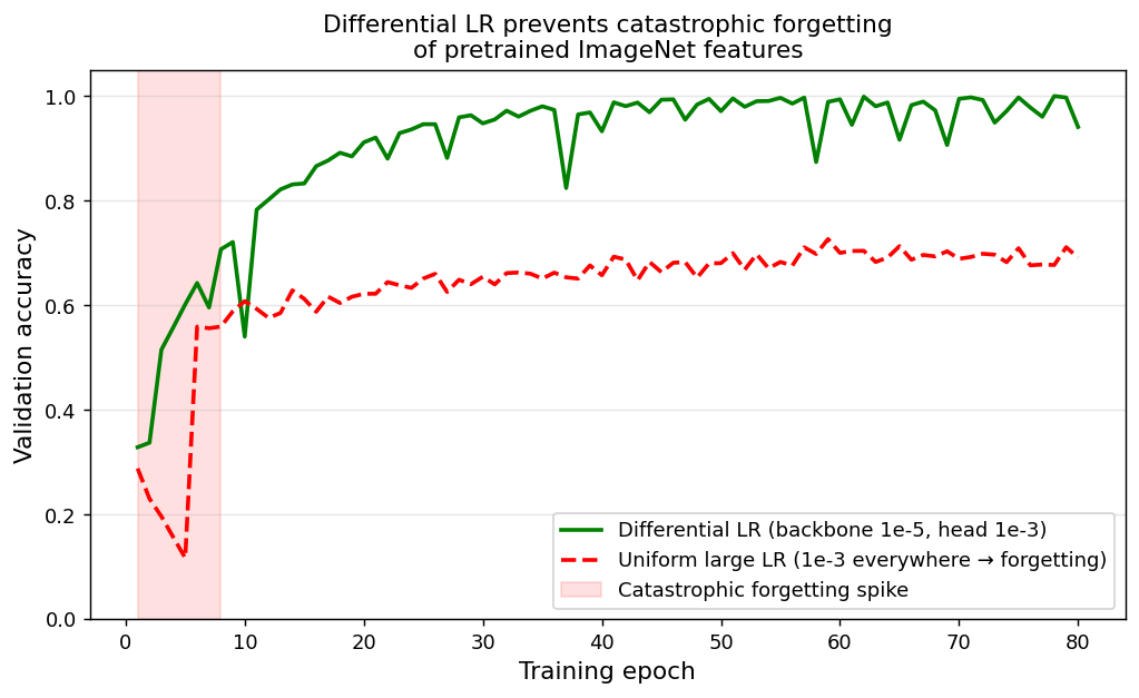
Validation accuracy during fine-tuning. Green (correct): differential LRs — backbone gets lr=1e-5, head gets lr=1e-3; accuracy climbs steadily. Red dashed (wrong): uniform large lr=1e-3 for the whole network — the first few epochs destroy pretrained ImageNet features (catastrophic forgetting spike); recovery is partial and slow.

Catastrophic forgetting mechanism: the randomly-initialised head produces large, near-random gradients in epoch 1. Backpropagated at the normal (large) lr through the pretrained backbone, these random gradients overwrite the carefully learned ImageNet features before the head has stabilised.
Differential learning rates: backbone lr ≈ $10^{-5}$; head lr ≈ $10^{-3}$ — a ratio of 100×.
The ratio reflects the distance to the minimum: the backbone is already at a good minimum (small steps needed); the head is randomly initialised far from any minimum (large steps needed).

The mechanism is the key exam concept: catastrophic forgetting is “a step size too large relative to the distance-to-good-minimum.” The backbone sits IN a good basin of the loss landscape. A large step hurls it out of that basin into random territory — you have destroyed your transfer in epoch 1.
Symptom of catastrophic forgetting: training loss spikes upward at the start of fine-tuning, or final accuracy is WORSE than feature-extraction despite theoretically having “more capacity.”
The 100× ratio is defensible: if head lr = 1e-3 and backbone lr = 1e-5, the backbone takes steps 100× smaller. In the loss-landscape picture: the backbone is near its minimum; the head is far from its minimum. Larger ratio = more conservative backbone.
Misconception to preempt: “can I fix catastrophic forgetting by using a smaller learning rate for everything?” Then the head never learns (it is far from its minimum and you have crippled it). The fix is ASYMMETRIC rates, not uniformly small ones.
EM anchor: in the notebook for this week, you will observe the catastrophic forgetting spike if you set backbone and head to the same lr. The fix is the two-parameter-group Adam.
Transition: “Transfer gives us pretrained features. Synthetic data gives us free labels.”

Gradual unfreezing prevents forgetting

Protocol (four stages):
1. Freeze all backbone layers. Train head at lr = $10^{-3}$ until validation plateau.
2. Unfreeze the last backbone block only. Train with backbone lr = $10^{-5}$, head lr = $10^{-3}$.
3. Unfreeze the next-to-last block. Reduce backbone lr slightly further.
4. Continue unfreezing from top to bottom (most domain-specific → most general).
The reason for top-down order: deepest layers are most domain-specific (need most adaptation) — unfreeze them first. Earliest layers are most general (preserve them longest).
Defence-in-depth: combine gradual unfreezing AND differential LRs. Do not choose between them. By keeping the backbone frozen until the head has converged, the backbone never sees random-gradient blasts.

Gradual unfreezing is the scheduled complement of differential LRs. Differential LRs control step size; gradual unfreezing controls timing. Together they provide defence-in-depth against catastrophic forgetting.
When to stop: unfreeze until validation loss stops improving. For most EM tasks with 50–200 images, you will stop after Stage 2 or 3 — the early backbone layers are so general that they do not need to change.
The one point to land: the head-first ordering is the Yosinski depth curve turned into a schedule. It is not arbitrary or magic — it follows from “the deepest layers are most domain-specific.”
Misconception to preempt: “gradual unfreezing is just slow.” The cost is more epochs — which in the small-data regime where overfitting is the real enemy, is almost always worth the trade. The fast path (unfreeze all at once) is only correct with abundant data.
Transition: “Now the materials-science superpower: synthetic data provides unlimited free labels.”

Synthetic data: free perfect labels by construction

The standard approach: acquire image → expert annotates label. Expensive, slow, limited.
The synthetic flip: choose label (the ground-truth structure) → render the image from it. The label is perfect by construction — no annotator disagreement, no boundary ambiguity, no label noise.
Materials advantage: we know the physics. Voronoi tessellations model grain topology. Phase-field simulations model microstructure evolution. Multislice simulations render realistic TEM images of known atomic structures Rakowski, Aaron et al., (2024).
Quantitative example: generating 10 000 Voronoi grain images takes minutes. Manually labelling 10 000 real SEM grain images takes months of expert time.
Caution: synthetic data fails on exactly the feature the generator omits. If Voronoi cannot make twins, a twin-detection model trained on it cannot learn twins — not a tuning problem but an epistemic one.

The labelling-arrow-flip is the central concept. In standard annotation: image → label (human provides). In synthetic: label → image (renderer provides). The label is not inferred; it is an input. This is why the mask is perfect.
The one point to land: synthetic data converts the labelling problem into a modelling problem. You no longer need someone to label real images, but your model is only as good as your generator’s physics — and it fails precisely on whatever feature the generator omits.
Misconception to preempt: “synthetic data always looks unrealistic and models trained on it will fail on real data.” This is sometimes true (the sim-to-real gap, covered next) but often false for grain topology tasks, as the case study shows.
EM anchor: the Construction Zone pipeline (Rakowski et al., npj Comput. Mater. 2024): thousands of random Au nanoparticles on carbon, rendered with multislice simulations including thermal effects, aberrations, plasmon losses, and Poisson dose noise → segmentation masks by construction. A U-Net trained ONLY on this synthetic data beat all previous models trained on real annotated TEM images on three benchmarks.
Transition: “The Voronoi tessellation is the simplest and most effective grain generator.”

Voronoi synthetic microstructure pipeline

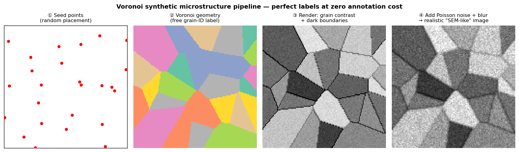
Voronoi synthetic microstructure pipeline for grain segmentation. From left: (1) random seed points placed in 2D; (2) each pixel assigned to its nearest seed — the Voronoi geometry gives perfect free grain-ID labels; (3) random intensity per grain + dark boundary strip renders a simple grain image; (4) Poisson noise + Gaussian blur makes it look like a low-magnification SEM acquisition.

Walk through the four panels. “Step 1: scatter N random seed points. Step 2: assign each pixel to its nearest seed — the Voronoi diagram. Every pixel’s grain ID is known by construction — that is the free mask. Step 3: give each grain a random intensity and darken the boundary pixels — now it looks like a grain-contrast SEM. Step 4: add Poisson noise and slight defocus blur — now it looks like a low-dose SEM acquisition.”
The one point to land: the mask is perfect because WE chose where the grains are. The renderer creates the image FROM the mask, not the other way around.
Caveat to state: Voronoi generates convex, roughly equiaxed grains with near-120° triple junctions. Real microstructures have non-convex grains, annealing twins (straight parallel boundaries — Voronoi never produces these), and elongated/columnar morphologies. The generator’s omissions become the model’s blind spots.
EM anchor: a 30-line NumPy job can generate this. Show the pseudo-code: distribute N seed points, compute argmin of distance from each pixel to all seeds, that is the grain_id array. grain_intensity = np.random.uniform() indexed by grain_id. The whole pipeline is in the week’s notebook.
Transition: “Why does this actually work on real SEM images when the synthetic images look nothing like them? The topological truth.”

Why synthetic grain training transfers to real SEM images

Topological truth of grain networks: triple junctions have ~120° angles. Boundaries are continuous closed curves. Grains fill space without gaps. These properties hold in every polycrystalline material, alloy-independent.
Voronoi captures exactly the topological truth — the connectivity of boundaries and junctions. It does not capture twins, non-convex shapes, or grain-interior texture. But for grain-boundary detection, topology is the task-relevant invariant.
Result: a U-Net trained only on Voronoi images with no real SEM images in training correctly identifies grain boundaries on real polycrystalline SEM images — because the task reduces to “find the dark narrow strip between two bright regions,” and that description transfers across all imaging conditions.
The generalisable rule: synthetic data works when the generator captures the task-relevant invariant. It fails when the task depends on a feature the generator omits.
Application: grain-size measurement, triple-junction statistics, grain-shape quantification — all work. Annealing twin identification, specific texture components — do not work without real data or a physics-based generator.

This slide resolves the apparent contradiction between “synthetic data fails on what the generator omits” (true) and “Voronoi-trained U-Net works on real SEM” (also true). The reconciliation is the topological invariant. Say it aloud: both statements are true. Topology transfers; twins do not.
The one point to land: the generalisable rule is the exam-grade understanding. “Synthetic data succeeds when the downstream task only needs the structure your generator gets right.”
Misconception to preempt: “if synthetic training worked for grain boundaries, it will work for everything.” No. It worked because grain-boundary topology genuinely is captured by Voronoi. For defect identification, phase fraction quantification, or twin detection, the generator would need to be more physically sophisticated.
EM anchor: the practical value is enormous. Generating 10 000 Voronoi images takes minutes on a laptop. 10 000 real labelled SEM grain images would take months of a postdoc’s time. The synthetic approach democratises labelled data creation for grain segmentation.
Transition: “The catch is the sim-to-real gap.”

The sim-to-real gap

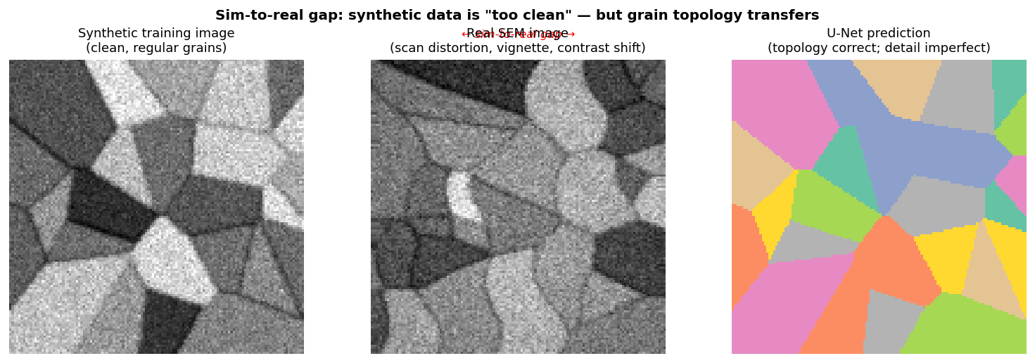
Three panels showing the sim-to-real challenge. Left: synthetic training image (clean, regular grains, no scan artefacts). Centre: real SEM image with scan distortion, vignette, and contrast drift relative to the synthetic distribution. Right: U-Net prediction — grain topology is correctly identified despite the gap, because topology is the task-relevant invariant.

The gap between synthetic and real is not just visual. It is statistical: the distribution of contrast, noise, spatial frequency content, and scan artefacts differs between what the generator produces and what the real instrument produces. A model trained on synthetic and tested on real sees a distribution shift at every pixel.
The one point to land: synthetic data fails exactly on the feature the generator omits. The model cannot learn what was never in the training set.
Walk through the three panels: “Left: clean synthetic. The model has only ever seen this. Centre: real SEM — same physical grain structure but different noise statistics, scan distortion, vignette. The model has never seen these. Right: the U-Net prediction correctly identifies grain boundaries despite the gap. Why? Because boundary topology (dark narrow strip separating two regions) is robust to all these transformations.”
Misconception to preempt: “domain shift always breaks synthetic-to-real transfer.” Not when the task depends only on features the generator captures correctly. For grain topology: it works. For anything more subtle: expect the gap to hurt.
Transition: “How do we close the gap when topology alone is not enough?”

Closing the sim-to-real gap: domain adaptation

Realistic noise modelling (cheapest and most effective): measure the actual noise parameters of the target instrument (Poisson gain factor, Gaussian readout sigma). Use those in the rendering pipeline. Now synthetic images match real noise statistics.
Style transfer / CycleGAN: learn the “texture skin” of real SEM images and paint it onto synthetic geometry while preserving the exact free mask. Powerful but adds training instability and requires real unlabelled images.
Adversarial domain adaptation: train an encoder whose features are statistically indistinguishable between synthetic and real domains — a domain discriminator is trained adversarially. No real labels needed, but requires careful balancing.
Fine-tuning on a few real labels: even 10–20 real labelled images, fine-tuned onto a synthetic-pretrained model, usually beats all the above. Always try the boring solution first.
Augmentation bridges the gap for free: brightness jitter, Poisson noise, blur, elastic deformation in the rendering pipeline are all domain-adaptation moves — they expand the synthetic distribution toward the real one.

The hierarchy of solutions, in order of effort-to-result:
1. Match noise statistics → free, fast, usually closes most of the gap.
2. Augmentation in the rendering pipeline → same effort as Part 2; directly closes imaging-condition gap.
3. Fine-tuning on 10–20 real labels → a few hours; usually beats elaborate domain adaptation with zero real labels.
4. CycleGAN or adversarial DA → expensive, unstable, only worth it when truly zero real labels are available.
The one point to land: “try the boring solution first.” A team spent a month on a CycleGAN to bridge the gap; a colleague matched their accuracy in an afternoon by (a) measuring detector noise parameters and (b) fine-tuning on 20 real labelled images.
EM anchor: the “boring solution” in practice: measure the MTF of your SEM detector, fit a Poisson + Gaussian noise model to a uniform flat-field image, plug those parameters into the Voronoi rendering pipeline. Total cost: one flat-field acquisition and 10 minutes of Python.
Transition: “A smarter strategy for allocating annotation effort: active learning.”

Voronoi limits: what the generator cannot produce

What Voronoi gets right: space-filling topology; ~120° triple junctions; random grain-size distribution; boundary connectivity. These topological properties transfer to real grain boundary detection.
What Voronoi cannot generate:
- Annealing twins: straight parallel boundaries at exactly 60° misorientation — a common feature in FCC metals (austenite, copper, aluminium). Voronoi never produces exactly straight, parallel boundaries.
- Non-convex grain shapes: heavily deformed microstructures with elongated, interlocking grain morphologies.
- Grain-interior sub-structure: deformation bands, low-angle boundaries, orientation gradients within one grain.
- Phase-specific contrast: in multi-phase alloys, different phases have systematically different contrast from different crystal structure, not just random intensity variation.
The rule: the generator’s omissions become the model’s blind spots. Know your generator’s physics before deploying.

This slide is the necessary counterweight to the “Voronoi works” success story. The key sentence: “the generator’s omissions become the model’s blind spots.”
The one point to land: Voronoi is the right choice when the task depends on grain topology (boundary location, triple junction count, grain-size distribution). For tasks that require recognising specific grain morphologies, phases, or crystallographic features, a more physically faithful generator is needed.
EM anchor: in a Ti-6Al-4V SEM cross-section, the α-lamellar / β phase contrast is not random intensity variation — it is determined by crystallographic orientation and phase composition. A Voronoi generator with random intensities cannot represent this. A phase-field simulation that includes both phases would be needed.
Transition: “When topology alone is not enough, the sim-to-real gap requires active management.”

The sim-to-real gap: a failure scenario

Scenario: you train a CNN on Voronoi synthetic images to detect grain triple junctions. It achieves 96% accuracy on held-out synthetic data. Deployed on real SEM, it drops to 61%.
Differential diagnosis:
1. Geometry gap: Voronoi gives only convex ~equiaxed grains; real sample has elongated grains after rolling → the junction geometry looks different.
2. Missing artefacts: real SEM has charging streaks, contamination spots that look like triple junctions.
3. Contrast gap: per-grain contrast model is too uniform; real grains have sub-grain structure from channelling.
4. Synthetic-style shortcut: model learned the Voronoi boundary-width regularities that are absent in real images.
The fix is not “more synthetic data” — more of a distribution that omits real artefacts still omits them. The fix is: add realistic rendering + fine-tune on 10–20 real images.

Run this scenario as a discussion question before revealing the differential diagnosis. Ask: “96% synthetic, 61% real — what went wrong?” The intended answer is: enumerate the four causes and distinguish them experimentally. Cause 1: test on equiaxed subset of real sample — if accuracy recovers, geometry gap confirmed. Cause 2: mask or simulate artefacts. Cause 3: add grain-interior texture to the rendering pipeline. Cause 4: Grad-CAM check — if saliency lights up on boundary width not boundary presence, it is a shortcut.
The misconception to surface: “add more synthetic data.” More of the wrong distribution does not help. The fix is closing the distribution gap — which requires understanding what the gap IS.
This is a callback to the Week 4 leakage lesson: same failure mode (model learns a spurious feature that is perfectly predictive in training but absent in deployment), different context (synthetic-style fingerprint vs specimen identity).

Active learning: label the most informative samples

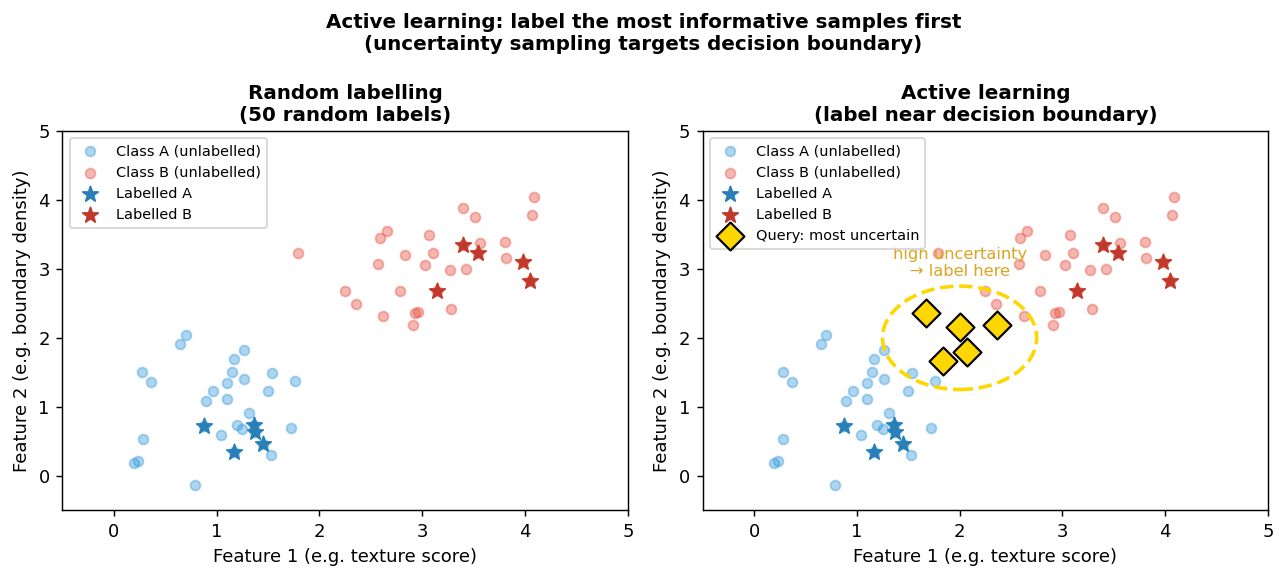
Left: random labelling strategy — 50 labels scattered uniformly across feature space. Right: active learning — labels concentrated near the decision boundary, where uncertainty is highest. With the same 50 labels, the active strategy correctly identifies the decision boundary; random labelling leaves a large uncertain region.

Active learning is the right tool when labels (not images) are the bottleneck. Materials science perfectly fits this condition: unlabelled SEM images can be acquired by the thousand in an automated session; what is scarce is expert annotation time.
The two strategies: (1) uncertainty sampling — label where the model is least confident (highest entropy, smallest margin); (2) diversity sampling — label points most different from already-labelled data (covers input space, avoids redundancy). Best practice combines both: uncertain AND diverse.
The one point to land: 50 strategically chosen labels can beat 500 random ones. Not always, but often by a large margin when the task has a clear decision boundary that random sampling covers poorly.
Misconception to preempt: “active learning always wins over random.” Not guaranteed. On some problems the decision boundary is uniformly distributed in feature space and active learning barely beats random. Present it as a high-leverage tool, not a free lunch.
EM anchor: in an automated TEM session on a new alloy, you acquire 500 diffraction patterns. Expert annotation budget: 30 patterns. Random choice: label 30 uniformly. Active choice: run the current model on all 500, pick the 30 where the predicted phase confidence is lowest. Then retrain and repeat.
Transition: “Let me put all three strategies together into a practical workflow.”

Active learning: the annotation loop

Step 1 — Seed: label a small random batch (10–20 images) to get a starting model.
Step 2 — Score: run the current model on all unlabelled images, compute an uncertainty score (e.g. entropy of class probabilities, or predictive variance).
Step 3 — Query: select the $k$ most uncertain images (or a mix of uncertain + diverse) for expert annotation.
Step 4 — Retrain: add newly labelled images to the training set, retrain (or fine-tune), return to Step 2.
Cold-start warning: with no initial labels the model’s uncertainty is meaningless (all predictions are near-chance). Always seed with a small random batch before activating uncertainty sampling.
Batch diversity trap: pure uncertainty sampling in batches picks a tight cluster of near-identical hard cases. Combine uncertainty with diversity (spread queries across feature space).

Cross-material transfer: when the source is another alloy

Strategy: pretrain on a large database of labelled images from one material system, then fine-tune on a small set from a different (but related) material.
Example: a grain-boundary segmentation model trained on 1 000 labelled steel SEM images is fine-tuned on 30 labelled aluminium SEM images.
Why this works: grain-boundary topology is alloy-independent — space-filling cellular networks with ~120° triple junctions appear in every polycrystalline metal. Contrast mechanisms differ (steel vs Al etch response), but the topological discriminant is the same.
Advantage over ImageNet: same imaging modality (SEM), same spatial scale, same task — much smaller domain gap than ImageNet → EM. Expect less fine-tuning and fewer target labels to reach the same accuracy.
Practical corollary: if a large labelled dataset exists for material A, it is worth fine-tuning for material B even if B seems very different. The shared topology is more powerful than the contrast difference is harmful.

The complete small-data EM workflow

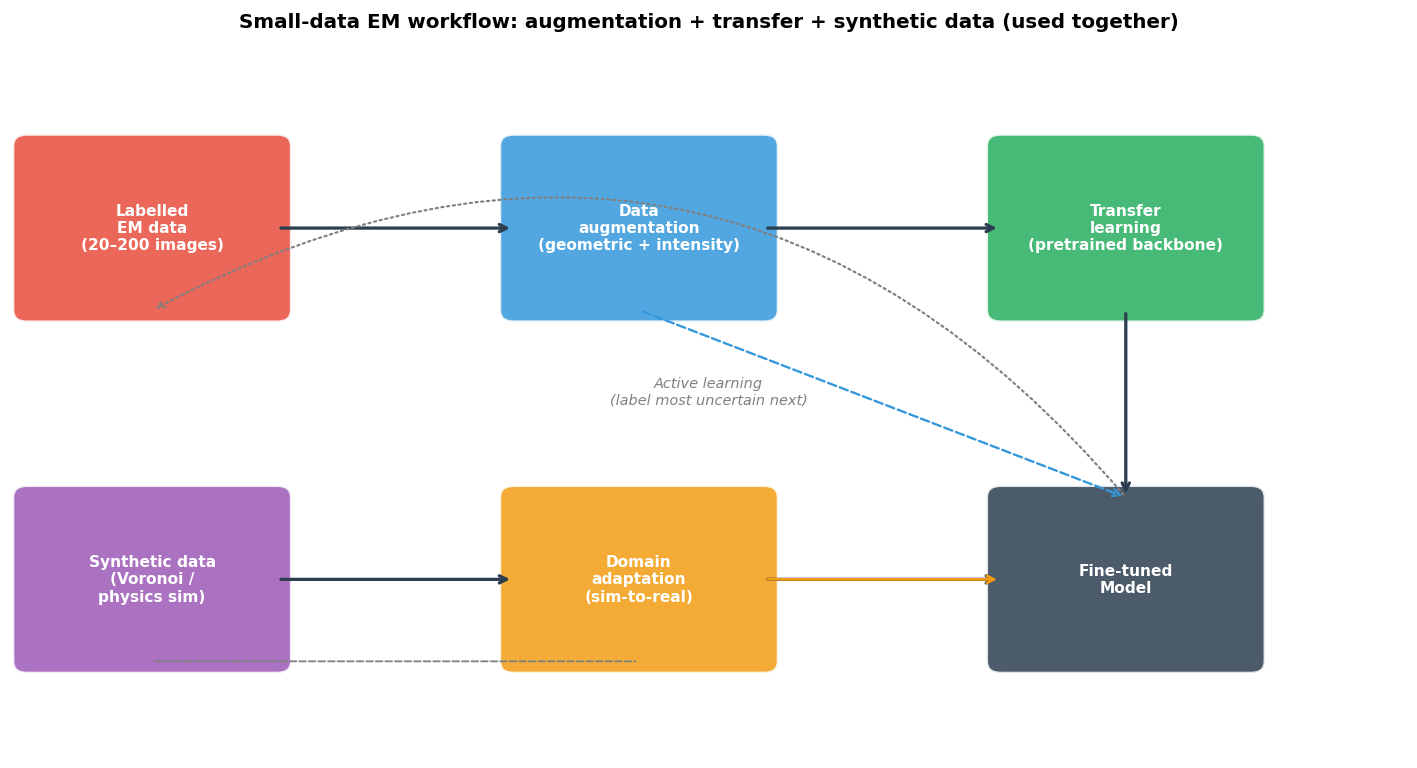
Complete small-data EM workflow diagram. The labelled EM data (20–200 images) feeds augmentation and transfer learning in parallel; synthetic data feeds domain adaptation; all three converge on a fine-tuned model. The active learning loop (dotted arrow, bottom) queries the fine-tuned model for the most uncertain unlabelled images, sends them to expert annotation, and grows the labelled pool.

Walk through the diagram explicitly: “We start with a very small labelled set. Simultaneously: augmentation manufactures more views of those labels; transfer learning imports features from ImageNet or a materials-pretrained model; synthetic Voronoi data provides thousands of free labels for pre-training. All three converge on one fine-tuned model. The active learning loop (dotted) then asks the model ‘which unlabelled images are you least confident about?’ and sends those to the expert annotator first.”
The one point to land: these are not alternatives — they are stacked. Every production EM segmentation pipeline uses at least two of the three legs. The strongest pipelines use all three.
Misconception to preempt: “I should pick the strategy that matches my situation.” Wrong framing. The three strategies are orthogonal and composable — they do not compete. Adding any one of them strictly improves over baseline; adding all three multiplies the benefit.
Forward link: Week 8 introduces autoencoders as unsupervised feature extractors — a fourth strategy for learning representations from unlabelled data. Autoencoders can pre-train a backbone on your own unlabelled micrographs, closing the ImageNet domain gap without requiring any labels at all.

Transfer learning in EM: published evidence

ImageNet → Au nanoparticle TEM segmentation Rakowski, Aaron et al., (2024): a U-Net with an ImageNet-pretrained ResNet encoder was fine-tuned on a small set of labelled TEM frames of Au nanoparticles on amorphous carbon. The pretrained encoder correctly identified “structured lattice fringe region vs featureless speckle” because that is a generic edge/texture discrimination task — exactly what ImageNet Layer 1–2 features are good at.
Voronoi → real SEM grain boundary detection Holm, Elizabeth A. et al., (2020); DeCost, Brian L. et al., (2017): a U-Net Ronneberger, Olaf et al., (2015) trained only on Voronoi synthetic images with no real SEM data in training correctly segments grain boundaries on real polycrystalline SEM images, because grain-boundary topology (dark thin strip between two regions) is the task-relevant invariant captured by Voronoi.
Key lesson from both examples: what transfers is not “knowledge about the specific objects.” What transfers is the visual vocabulary — edge detectors, contrast-change detectors, texture detectors — which is universal across image domains and across synthetic-to-real transfer Goodfellow, Ian et al., (2016).
The common pattern: both succeeded because the task reduced to a generic visual discrimination (structured vs unstructured; boundary vs interior) rather than a domain-specific one (specific crystal structure, specific defect type).

Validation in the small-data regime

Group by specimen, not by crop: if crops from the same EM specimen appear in both train and test, the model memorises specimen identity (detector vignette, brightness baseline, session contrast) rather than the physical microstructure.
The protocol: GroupKFold(n_splits=5).split(X, y, groups=specimen_ids) — entire specimens are in either train or test, never both. This is the Week 4 lesson applied to the augmented EM context.
Augmentation leakage: if you augment before splitting, a rotated copy of a training image lands in the test set. The test accuracy measures memorisation recall, not generalisation. Rule: split first, then augment.
Honest consequence: group-based splitting gives lower and noisier numbers — with 5 specimens your effective test set is 2 specimens. That lower honest number beats a higher leaked one every time. The variance is information (it tells you how little you actually know), not a problem to optimise away.

Practical checklist for small-data EM tasks

Before augmenting: confirm each transform is physically valid for your specific material and task. If the label is calibrated to intensity, brightness jitter is illegal.
Always GroupKFold by specimen (not by crop): split first, then augment. A rotated copy of a training specimen must not appear in the test set.
Start with feature extraction (<100 labels): freeze backbone, train only head. If accuracy is too low, move to fine-tuning with differential LRs.
Synthetic pre-training: if you have a physical model of your microstructure, generate 1 000–10 000 synthetic images first. Even simple Voronoi geometry pre-training helps if the task depends on topology.
Fine-tune with differential LRs: backbone lr $\approx 10^{-5}$, head lr $\approx 10^{-3}$. Use gradual unfreezing (head → last block → deeper blocks).
Active learning: if you can acquire unlabelled images cheaply, prioritise annotation budget on the most uncertain ones — uncertainty sampling or entropy scoring.

Use this as the practical recipe students will carry into their miniproject. Point out that the first two bullets are validation hygiene that overrides everything else — a perfect three-strategy pipeline with a leaky split produces a confidently wrong model.
The one point to land: GroupKFold by specimen is not optional hygiene — it is the difference between a number you can publish and a number that is a lie. This is Week 4’s lesson revisited in the small-data EM context.
EM anchor: “start with feature extraction” is the practical rule for the typical EM lab situation. With 30 labelled images and a ResNet-50 backbone, feature extraction (train only the head) avoids overfitting the backbone and gives a working model within minutes. Fine-tuning is the next step once the head has converged.

Quantitative summary: what each strategy delivers

Strategy	Label budget	Typical gain	Key caveat
Augmentation alone	50 images	$$1.5–3× effective data	Invalid transforms hurt
Feature extraction	20–100 images	$$10–30% accuracy improvement	BN running stats trap
Full fine-tuning	100–1000 images	$$20–50% over scratch	Catastrophic forgetting if no diff-LR
Voronoi pre-train	0 real labels	Strong baseline for grain tasks	Fails for twins, non-equiaxed
All combined	20–50 real labels	Close to full-data performance	Honest grouped validation required

Use this table as a mini-summary before the forward link. Ask students to justify each entry from the slides.
The key row is the last one: all combined, 20–50 real labels can approach the accuracy of a fully-supervised model with 500 labels. That is the main message of this week.
Misconception to preempt: “feature extraction is always enough.” With a large ImageNet-EM domain gap (e.g. 4D-STEM diffraction patterns, which look nothing like natural images), the features may need meaningful adaptation — fine-tuning on 200 real images will outperform frozen feature extraction.
The BN running stats trap: a frozen backbone put in eval() mode uses ImageNet’s stored batch normalisation statistics. Grayscale 16-bit micrographs have completely different statistics. Fix: keep BN layers in training mode even when backbone weights are frozen.
Transition: “Let us close with the forward link to Week 8.”

Putting it all together: the Voronoi → SEM grain segmentation pipeline

Step 1 — Synthetic pre-training: generate 5 000 Voronoi grain images in minutes; train a U-Net on them. The encoder learns grain topology features for free.
Step 2 — Augmentation: during pre-training, apply random intensity jitter, Poisson noise, elastic deformation, random crops. The encoder becomes robust to contrast and scale variation.
Step 3 — Fine-tune on real SEM images: collect 30 expert-labelled real SEM grain images. Fine-tune: freeze encoder (feature extraction) → train decoder and skip connections at high LR → unfreeze encoder at low LR.
Step 4 — Honest validation: split 30 images by specimen (not by crop). Report IoU and Dice on the held-out specimens, not accuracy.
Result: a grain-segmentation U-Net that generalises across imaging sessions, magnifications, and grain sizes — using only 30 labelled real images and no ImageNet.
Connect to Week 6: the U-Net architecture (encoder-decoder with skip connections) is unchanged from last week. What changed is how we train it.

Forward link: Week 8 — Unsupervised learning and autoencoders

Today’s remaining gap: transfer learning from ImageNet imports features learned on natural photographs (dogs, cars, buildings). The domain gap to EM data (atomic-resolution HAADF, diffraction patterns, EELS maps) is real.
Week 8’s answer: an autoencoder learns representations from your own unlabelled EM data — no ImageNet needed, no labels needed, no synthetic generator needed. It compresses each image into a compact latent vector and reconstructs it, learning the features that matter most for your data.
Why this is powerful: a backbone pre-trained with an autoencoder on 10 000 unlabelled EM images will have features far better matched to your microscopy task than an ImageNet backbone — and requires zero annotation.
Autoencoders also enable: anomaly detection (reconstruction error flags unusual images), dimensionality reduction for exploring large datasets, and latent-space interpolation for controlled microstructure generation.
The connection: augmentation + transfer + synthetic (today) PLUS unsupervised pre-training on unlabelled EM data (Week 8) is the complete modern small-data toolkit.

Close the forward link explicitly. “Today we imported knowledge from ImageNet and from synthetic generators. Both involve either a domain gap (ImageNet) or a physics approximation (Voronoi). Week 8 closes both by learning directly from your unlabelled EM data.”
The one point to land: autoencoders do not require labels. They are the fourth lever in the small-data toolkit, and for EM modalities with a large ImageNet domain gap (diffraction, EELS, 4D-STEM), they are often the most powerful baseline.
Misconception to preempt: “autoencoders are just for denoising.” They have many uses — compression, anomaly detection, latent-space control, and as backbone pre-trainers. Denoising is one use case, not the whole picture.
EM anchor: an autoencoder pre-trained on 5000 unlabelled HAADF images from your specific microscope will learn the contrast statistics, noise level, and typical feature scales of that instrument. A downstream U-Net initialised from this backbone will converge faster and with fewer labelled images than one starting from ImageNet.
Pacing note: this is the closing slide — 3 minutes maximum. Set up Week 8 as the natural continuation and close with enthusiasm.

Continue

→ Next: Week 08 — Unsupervised learning & autoencoders for EM
← Back: Week 06 — CNNs for microscopy images
All courses

References

Overview: Computer vision and machine learning for microstructural characterization and analysis, Metallurgical and Materials Transactions A, Elizabeth A. Holm & others.

Materials data science, Stefan Sandfeld & others.

How transferable are features in deep neural networks?, Advances in neural information processing systems, Jason Yosinski, Jeff Clune, Yoshua Bengio, & Hod Lipson.

Deep residual learning for image recognition, Proceedings of the IEEE conference on computer vision and pattern recognition, Kaiming He, Xiangyu Zhang, Shaoqing Ren, & Jian Sun.

Construction zone: A machine learning dataset and benchmark for training and evaluating HRTEM nanoparticle segmentation algorithms, npj Computational Materials, Aaron Rakowski & others.

Exploring the microstructure manifold: Image texture representations applied to ultrahigh carbon steel microstructures, Acta Materialia, Brian L. DeCost & Elizabeth A. Holm.

U-net: Convolutional networks for biomedical image segmentation, Medical image computing and computer-assisted intervention (MICCAI), Olaf Ronneberger, Philipp Fischer, & Thomas Brox.

Deep learning, Ian Goodfellow, Yoshua Bengio, & Aaron Courville.