Data Science for Electron Microscopy
Week 8: Unsupervised learning & autoencoders for EM

Prof. Dr. Philipp Pelz

FAU Erlangen-Nürnberg

Institute of Micro- and Nanostructure Research

Recap: Week 7 and today’s question

• Week 7: three strategies for beating the labelled-data bottleneck — data augmentation, transfer learning from ImageNet, and Voronoi synthetic pre-training.
• Core insight: transfer learning imports features learned elsewhere and fine-tunes them; but ImageNet features carry a real domain gap to EM data (diffraction patterns, EELS maps, atomic-resolution HAADF look nothing like dogs or cars).
• The remaining gap: what if we have 10 000 unlabelled EELS spectra from our own microscope — no labels, no ImageNet, no synthetic generator — and we want to extract chemical information from them?
• Today’s answer: unsupervised learning. We do not need labels to find structure. The data itself provides the supervisory signal.
• Concrete payoff: a denoising autoencoder trained on low-dose spectra recovers clean peak shapes; its latent space clusters iron-oxide phases with no labels; anomalous spectra (damaged regions, contamination) stand out by high reconstruction error.

• Open by closing the loop from Week 7: “last week we answered the label bottleneck with three external sources of knowledge — ImageNet, Voronoi, augmentation. Today we answer it with our own data.”
• Make the domain-gap concrete: show of hands — how many think a ResNet trained on dogs detects Fe³⁺ vs Fe²⁺ in an EELS fine structure? That is the gap an autoencoder closes by learning from your own spectra.
• Pacing: 3 minutes maximum. The key phrase to land: “the data is the label — we ask it to reconstruct itself.”
• Transition: “Let me show the roadmap and then the key motivating example.”

Road map and self-study

• Road map: recap Week 7 + today’s question (2) · unsupervised learning landscape — what and why (3) · k-means: Lloyd’s algorithm, initialization, choosing K, failure modes, practical tips (5) · GMM as soft clustering (3) · manifold hypothesis and why compression works (3) · autoencoders: architecture, reconstruction, PyTorch, bottleneck choice (4) · linear AE ≈ PCA; nonlinear AE beyond PCA (3) · denoising autoencoders for low-dose EELS/EDS (4) · latent space: t-SNE/UMAP visualization and phase clustering (4) · anomaly/novelty detection by reconstruction error and latent outliers (3) · VAE conceptual preview — rVAE for STEM; full math Week 12 (3) · putting it together + forward link to Week 9 (3) — 40 content slides total (within the 40–48 target).
• Self-study: notebooks/week08_denoising_autoencoder.ipynb — build synthetic noisy EELS-like spectra, train a small denoising autoencoder on CPU in under 2 minutes, compare AE vs PCA denoising, visualise latent-space phase clusters, and explore the effect of bottleneck dimension in the exercise.

• Read the roadmap at medium pace. The two anchors to call out: denoising for low-dose spectra (the practical payoff) and anomaly detection (another zero-label application). Both have no parallel in supervised learning.
• One pacing note: this slide is orientation only — 1 minute. Do not read every bullet. Gesture at the structure and move forward.
• Transition: “Start with the big picture — why unsupervised at all.”

The unsupervised learning landscape

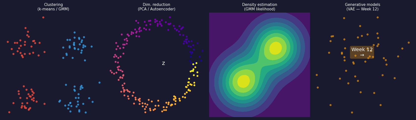
The four families of unsupervised learning. Clustering assigns each spectrum to a discrete group (k-means, GMM). Dimensionality reduction finds a low-dimensional coordinate that summarises each spectrum (PCA, autoencoder). Density estimation models the full probability distribution over spectra. Generative models sample new spectra from that distribution — introduced as a teaser for Week 12.

• Walk through the four quadrants left to right.
• The boundary between dimensionality reduction and generative modelling is where the VAE lives; that is Week 12.
• The two tasks we will develop today are clustering (k-means, GMM) and dimensionality reduction (autoencoder). They are not alternatives — they work together: an autoencoder reduces dimension, then k-means clusters the latent codes.
• Transition: “Why does any of this matter for EM? Labels.”

Why unsupervised matters for electron microscopy

• Most EM data arrives unlabelled. A 4D-STEM scan is hundreds of GB of diffraction patterns; an EELS map is millions of spectra. None of them come with a label until a human expert provides one.
• Clustering for exploration: before you can label, you need a hypothesis. Unsupervised clustering of spectra surfaces candidate phases for a domain expert to inspect.
• Compression for speed: a 1024-channel EELS spectrum can be compressed to 8 latent numbers without losing chemical content — enabling interactive visualisation of maps that would otherwise be too slow to display.
• Anomaly detection for quality control: spectra from contaminated regions, beam-damaged areas, or novel chemistry reconstruct poorly from an AE trained on normal data — flagged automatically, at zero annotation cost.
• The rule of thumb: if you have no labels at all, start with PCA to understand dimensionality, then an AE to capture non-linear structure Sandfeld, Stefan et al., (2024).

• Hammer the “labels are expensive” point from Week 7 but now flip the perspective: instead of reducing the label requirement, we eliminate it entirely.
• EM anchor: a real EELS map from an iron-oxide thin film: 128×128 pixels × 1024 energy channels = 16 million numbers. The domain expert knows there are probably three phases (Fe₂O₃, FeO, Fe₃O₄). Clustering the 16 384 spectra by their latent codes recovers those three phases without any labels — confirming the hypothesis in minutes instead of hours of manual peak fitting.
• Transition: “Start with the simplest clustering algorithm — k-means.”

Unsupervised methods and their EM applications

• K-means: fast geometric clustering of spectral vectors or latent codes. Phase maps from EELS, EDS phase identification. Output: hard cluster labels (each spectrum belongs to one phase) Bruefach, Alexandra et al., (2023), doi:10.1063/5.0130546.
• GMM: soft probabilistic clustering — boundary spectra get a mixture of responsibilities. Better for overlapping phases (e.g., Fe₂⁺/Fe³⁺ mixtures).
• PCA: linear dimensionality reduction; Week 3 foundation. Decomposes a spectral map into orthogonal “eigenspectra” and abundance maps. Fast, interpretable, assumes linear mixing.
• Autoencoder: non-linear generalization of PCA. Learns curved manifolds — peak shifts, fine-structure changes, non-linear mixing. Today’s main topic.
• t-SNE / UMAP: visualize high-dimensional latent codes in 2D. Diagnostic tool for latent space quality; not a dimensionality reduction method for downstream tasks.

• The hierarchy matters: PCA is a special case of a linear AE; k-means clustering of latent codes is downstream of the AE. Give the students the mental model of a pipeline: raw spectra → AE → latent codes → clustering.
• Transition: “Build up k-means from first principles — it is the workhorse.”

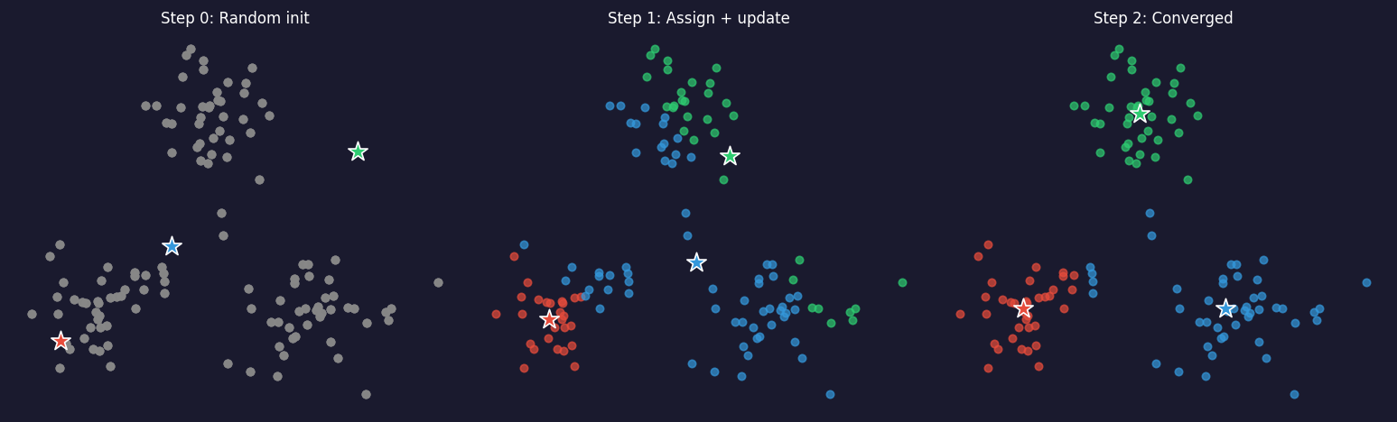
K-means: objective and Lloyd’s algorithm

Assign \(N\) spectra \(\{x_1, \ldots, x_N\} \subset \mathbb{R}^d\) to \(K\) groups \(C_1, \ldots, C_K\) by minimising:

\[ J = \sum_{k=1}^{K} \sum_{x_i \in C_k} \|x_i - \mu_k\|^2. \]

Lloyd’s algorithm — alternate two steps until assignments stop changing:

1. Assign: each spectrum goes to its nearest centroid \(\mu_k\).
2. Update: each centroid moves to the mean of its assigned spectra.

Each step strictly decreases \(J\); convergence in finitely many steps is guaranteed — to a local minimum.

Three steps of Lloyd’s algorithm on a toy two-dimensional dataset. Stars mark centroids (initially random, then updated). After two assign–update cycles the centroids have settled on the true cluster centres. The same logic applies to clustering 1024-D EELS spectra; only the distance computation changes dimensionality.

• K-means is coordinate descent on \(J\): hold centroids fixed → solve for assignments; hold assignments fixed → solve for centroids. Each subproblem has a closed-form solution (nearest centroid; mean).
• Critical limitation to name now: K-means uses Euclidean distance, which requires that distance is meaningful in the feature space. For raw 1024-D EELS spectra, Euclidean distance is dominated by the highest-intensity region (the zero-loss peak). Always normalise or, better, cluster latent codes rather than raw spectra.
• Transition: “The local minimum problem motivates smart initialization.”

K-means: initialization and K-means++

• The problem: random initialization can place two centroids in the same cluster and miss another entirely. Different random starts give different final clusterings.
• K-means++ (standard default in scikit-learn) solves this:
  1. Pick the first centroid uniformly at random.
  2. Pick each subsequent centroid with probability proportional to \(D(x)^2\) — the squared distance to the nearest already-chosen centroid.
  3. This spreads the initial centroids, giving a provably better expected final \(J\).
• Practical recipe: use K-means++ plus 5–10 random restarts; keep the run with lowest \(J\).
• EM application: clustering latent codes (8-D AE output) rather than raw spectra (1024-D) makes K-means dramatically faster and more stable — the latent space is better conditioned Bruefach, Alexandra et al., (2023), doi:10.1063/5.0130546.

• The \(D(x)^2\) weighting is the key: it gives far-away points much higher probability of becoming a seed, so seeds naturally spread over different regions.
• The “cluster latent codes not raw spectra” point is the practical payoff of the whole lecture: AE first, then cluster. This is the standard pipeline in computational EM.
• Transition: “Choosing K is separate from finding the clusters — let me show the two standard diagnostics.”

Choosing K: elbow method and silhouette score

Elbow method: - Run k-means for \(K = 1, 2, \ldots, K_{\max}\). - Plot \(J(K)\) vs \(K\). Look for the elbow: the point where \(J\) stops dropping fast. - Intuition: adding one more cluster beyond the true \(K\) gives diminishing returns.

Silhouette score: \[s(x_i) = \frac{b(x_i) - a(x_i)}{\max(a(x_i), b(x_i))}\] where \(a\) = mean intra-cluster distance, \(b\) = mean distance to nearest other cluster. Range: \([-1, 1]\), higher is better. Pick \(K\) that maximises mean silhouette.

Rule: use elbow and silhouette together. If they agree, more confidence.

• \(J(K)\) always decreases — at \(K = N\) every point is its own cluster and \(J = 0\).
• The elbow signals diminishing returns from extra clusters.
• Silhouette gives a per-point quality score: \(s > 0.5\) indicates good separation.
• Materials caveat: there is no objectively “correct” number of phases — the right \(K\) is the one a metallurgist or surface scientist can interpret. Use domain knowledge as a final sanity check.

• The elbow is sometimes obvious (sharp bend), often not (smooth curve). When it is ambiguous, use the silhouette.
• EM anchor: for an Fe–O thin film with three known iron-oxide phases, the elbow at K=3 and the silhouette peak at K=3 confirm the chemical expectation. A K=4 run would typically split one of the three phases into two sub-regions — real or artefact? Domain knowledge decides.
• Transition: “K-means gives hard assignments. GMM generalises to soft.”

K-means failure modes in EM data

• Spherical assumption: k-means uses Euclidean distance to a single centroid — implicitly assuming clusters are spherical and equal-sized. An elongated cluster (e.g., a phase with a peak that shifts continuously) is split incorrectly.
• Scale sensitivity: a single high-intensity spectral feature (zero-loss peak, characteristic X-ray line) dominates the Euclidean distance and swamps chemical differences. Fix: normalise each spectrum to unit peak or cluster latent codes.
• Outlier sensitivity: a single contaminated spectrum with extreme intensity pulls a centroid far from the true phase centre. Fix: remove outliers first (reconstruction-error threshold from the AE) or use K-medoids.
• No uncertainty: a spectrum on the boundary between two phases gets a hard label — but a human expert would call it “mixed.” GMM addresses this.

• The scale sensitivity is the most important practical failure mode. Students who cluster raw EELS spectra will almost always see this — the zero-loss peak dominates. The fix is to cluster AE latent codes (which are by construction normalised by the bottleneck) or PCA scores (which are variance-weighted).
• Transition: “GMM replaces the hard assignment with a soft probability.”

K-means in practice: the AE latent space is better to cluster

• Raw spectra (1024-D): Euclidean distance is dominated by the zero-loss peak and the absolute intensity level. Two spectra with the same chemistry but different sample thicknesses cluster differently — wrong.
• PCA scores (top-\(k\) components): variance-weighted projection. Better than raw, but linear. Minority phases with low total variance can be compressed into noise-floor components.
• AE latent codes (\(k\)-D): by definition, these \(k\) numbers are the most information-efficient representation the network found. They discard noise and capture chemical identity — the right things to cluster Peña, Francisco de la et al., (2019).
• Practical recipe for EM: (1) normalise each spectrum to unit peak intensity; (2) train denoising AE to \(k\)-D latent; (3) run k-means on latent codes; (4) visualise cluster centroids decoded back to spectrum space to verify chemical assignment.
• The rule: never cluster 1024-D raw spectra with k-means. Always reduce dimension first — PCA for a fast baseline, AE for the production pipeline.

• This is the most practical slide in the k-means section. It closes the loop: k-means is the workhorse, but what you feed it matters enormously. The AE latent space is the right input.
• EM anchor: two EELS spectra of FeO at 50 nm and 200 nm sample thickness. In raw 1024-D space, the zero-loss peak dominates — they cluster with different-chemistry but same-thickness spectra. In AE latent space, the thickness information has been absorbed into one latent dimension and the chemistry drives the clustering.
• Transition: “GMM replaces the hard assignment with a soft probability.”

GMM: soft clustering for overlapping phases

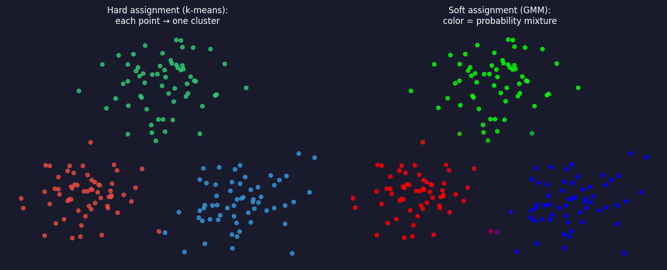
Hard vs soft assignment on the same spectral dataset. Left: k-means — each point belongs to exactly one phase (coloured circles). Right: GMM — each point carries a probability over phases; points near boundaries are shown as colour mixtures. This matters physically when EELS spectra from a transition zone contain contributions from both adjacent phases.

• The left panel is k-means: every point gets a single colour. The right panel is GMM: boundary points are colour-mixed — they carry probability mass in two clusters. This is physically meaningful for EM data where phase boundaries are several unit cells wide.
• Transition: “Let me state the GMM concisely without the full EM derivation — we want the intuition.”

GMM: the model and the key intuition

A weighted sum of \(K\) Gaussian densities: \[ p(x) = \sum_{k=1}^{K} \pi_k \,\mathcal{N}(x;\,\mu_k,\,\Sigma_k), \quad \sum_k \pi_k = 1. \]

Intuition: each phase \(k\) is modelled as a Gaussian cloud of spectra centred on the phase-representative spectrum \(\mu_k\) with a covariance \(\Sigma_k\) encoding spectral variability.

Soft assignment (responsibility): \[\gamma_{ik} = P(\text{phase } k \mid x_i) \propto \pi_k\,\mathcal{N}(x_i;\,\mu_k,\Sigma_k).\]

• K-means vs GMM: same goal, different shape. K-means allows only spherical clusters; GMM allows ellipsoidal clusters of any orientation.
• EM payoff: an Fe₂O₃ phase may have higher variance along the Fe-L₂₃ edge than along the O-K edge. A full-covariance GMM captures this anisotropy; k-means cannot.
• Fitting: alternating E-step (compute \(\gamma_{ik}\)) and M-step (update \(\mu_k, \Sigma_k, \pi_k\)). No full EM derivation needed here — the intuition is alternating between “which phase does this spectrum belong to?” and “what is each phase’s average spectrum?”.

• Do not derive EM. The exam expects the student to state (1) what a responsibility is (soft probability), (2) what the E- and M-steps do qualitatively, (3) that GMM generalises k-means by allowing ellipsoidal clusters.
• Practical note: in high dimensions (1024-D raw spectra), full covariance GMM has too many parameters. Use diagonal covariance or, again, cluster latent codes in a low-D space where full covariance is feasible.
• Transition: “Both k-means and GMM cluster in whatever space you give them. The quality of the clustering depends on the quality of the space. That is the manifold hypothesis.”

K-means vs GMM: comparison table

	K-means	GMM
Assignment	hard (one cluster)	soft (probability vector)
Cluster shape	spherical	ellipsoidal (full \(\Sigma\))
Speed	fast	slower (covariance update)
Boundary handling	abrupt	smooth
Choosing \(K\)	elbow + silhouette	BIC (penalised log-likelihood)
High-dim risk	Euclidean dominance	covariance explosion (\(d^2\) params)

Rule of thumb: k-means for fast exploration; GMM when clusters overlap, vary in shape, or you need probabilities for downstream decisions. In both cases, prefer clustering latent codes over raw spectra Murphy, Kevin P., (2012).

• Use this table as a quick orientation — it is an exam-style summary.
• The high-dim covariance explosion is the key practical reason to cluster latent codes. A 1024-D full-covariance matrix has ~500k parameters per phase — more parameters than data points.
• Transition: “Why does compression into a latent code work at all? The manifold hypothesis.”

The manifold hypothesis: why compression works

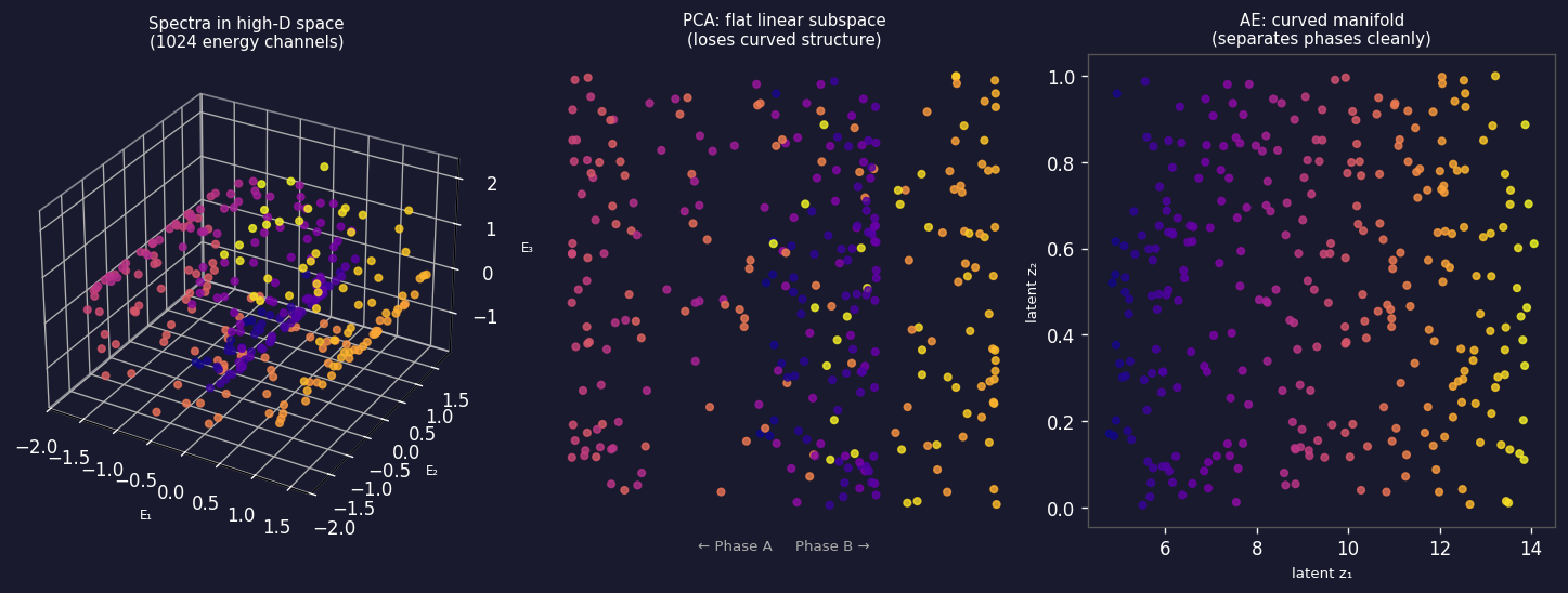
From high-dimensional spectra to a curved low-dimensional manifold. Left: three-dimensional view of data lying on a curved 2D surface embedded in 3D (analogy for 1024-D spectra on a ~10-D surface). Centre: PCA finds the best flat hyperplane — it unrolls the curve linearly and loses structure. Right: a nonlinear autoencoder follows the curved manifold, keeping phases separated along interpretable latent axes.

• The three-panel figure is the core pedagogical image. Walk through it carefully.
• Left: the data lives on a lower-dimensional surface — this is the manifold. For EELS data, the intrinsic dimension is close to the number of chemically distinct phases (3–5) plus the number of independent background parameters.
• Centre: PCA finds the flat hyperplane that minimises total reconstruction error. If the manifold is curved, the flat plane cuts through “holes” in the data. Phases that are separated on the manifold get pushed together by the linear projection.
• Right: an AE can bend its latent axes to follow the curve. Phases that were overlapping in the PCA view separate cleanly in the AE latent.
• Key numbers for EM: a 1024-channel EELS map of an iron-oxide film has intrinsic dimension ~3 (three iron-oxide phases). PCA needs 20–30 components to capture 95% of variance because noise is isotropic; an AE with 8 latent dimensions can separate all three phases while discarding noise.
• Transition: “An AE is the tool that implements manifold learning. Let me show how it works.”

Why the manifold dimension matters for EM spectra

• Physical argument: a pure-phase EELS spectrum is determined by a small number of physical parameters — elemental identity, oxidation state, bonding geometry, thickness. For a two-phase system these might be five numbers. Yet we measure 1024 energy channels.
• Consequence: 1024 channels – 5 physical degrees of freedom = ~1019 dimensions of noise and redundancy.
• PCA captures this as: variance explained by the first 5 components >> variance in remaining components. The “scree plot elbow” (Week 3) is a direct signature of the manifold dimension.
• Autoencoder advantage: PCA’s subspace is flat; a real spectral manifold is curved — oxidation-state changes cause non-linear peak-position and intensity changes. A nonlinear AE can represent this curved surface with fewer latent dimensions than PCA needs Goodfellow, Ian et al., (2016).
• Rule: if the scree plot elbow is at \(k\), try a bottleneck of \(k\) to \(2k\) in the AE.

• The “5 physical numbers” framing gives students an intuitive sanity check: if you have 3 known phases, a bottleneck of 3–8 is a reasonable starting point.
• The PCA–AE comparison is examinable: “PCA finds the best flat subspace; AE finds the best curved surface.”
• Transition: “Now build the autoencoder from its components.”

The manifold hypothesis in practice: 4D-STEM example

• Bruefach, Alexandra et al. (2023), doi:10.1063/5.0130546 applied clustering to 4D-STEM datasets of silver nanoparticles. Each diffraction pattern (128×128 pixels) lives in a 16 384-dimensional space.
• Observation: for a three-phase dataset (three crystallographic orientations), only a handful of principal components capture the orientation information; the rest is shot noise.
• Pipeline: PCA → keep top 10 components → k-means with \(K=3\) → phase map. Without PCA pre-compression, k-means fails because noise dominates Euclidean distance.
• The generalisation: replace PCA with an AE when orientations vary non-linearly (e.g., continuous tilt series). The AE latent space then smoothly parameterises orientation as a 1-D or 2-D latent coordinate.
• Lesson: always compress before clustering. Noise lives in all dimensions equally; signal lives in a low-dimensional manifold.

• The Bruefach paper is a directly citable EM case study. The three-phase Ag example makes the argument concrete: three orientations = intrinsic dimension 3; 16 384 diffraction-pattern channels; PCA pre-compression is essential.
• Transition: “Now build the autoencoder architecture.”

Autoencoder architecture: encoder–bottleneck–decoder

A deep autoencoder for spectral data. The encoder (blue, left) progressively compresses a 1024-channel spectrum to an 8-dimensional latent code z through successive hidden layers. The decoder (green, right) reconstructs the original 1024 channels from z. The bottleneck (red, centre) is the only constraint: it must retain enough information to reconstruct the input. The MSE reconstruction loss (orange, bottom) is the only supervisory signal — no labels needed.

• Walk through the hourglass architecture carefully. Count the layer widths: 1024 → 512 → 128 → 32 → 8 (bottleneck) → 32 → 128 → 512 → 1024. This is symmetric by convention.
• The key insight: the bottleneck forces the network to find a compact representation. Without the bottleneck, the trivial solution is the identity function. The bottleneck creates a useful constraint.
• Transition: “The training loop is standard PyTorch — one loss, one backward call.”

Autoencoder: the reconstruction objective

The autoencoder minimises: \[ \mathcal{L}(\theta, \phi) = \frac{1}{N}\sum_{i=1}^{N} \bigl\|x_i - g_\theta(f_\phi(x_i))\bigr\|^2. \]

• No labels — only the inputs themselves serve as targets. This is self-supervised: the supervisory signal is built into the data.

• Minimising \(\mathcal{L}\) forces the bottleneck \(z = f_\phi(x)\) to retain enough information to reconstruct \(x\). This is the minimum description length principle: compress as much as possible while losing as little as possible.

• In PyTorch (one line):

  loss = ((x - decoder(encoder(x)))**2).mean()

• For Poisson-noisy EM spectra: consider Poisson negative-log-likelihood as the loss instead of MSE, because pixel variance grows with the signal Sandfeld, Stefan et al., (2024).

• “Self-supervised” is the precise term: the label is derived from the data itself, not from an external annotator. This is how the AE escapes the labelling bottleneck.
• The Poisson loss note is a Week 2 callback: Gaussian noise → MSE; Poisson noise → Poisson NLL. Remind students that this is the same principle.
• Transition: “The simplest autoencoder — linear layers, no activations — turns out to be exactly PCA.”

Autoencoder in PyTorch: spectral data

import torch
import torch.nn as nn

class SpectralAE(nn.Module):
    def __init__(self, input_dim=128, latent_dim=8):
        super().__init__()
        self.encoder = nn.Sequential(
            nn.Linear(input_dim, 64), nn.ReLU(),
            nn.Linear(64, 32),        nn.ReLU(),
            nn.Linear(32, latent_dim)          # bottleneck — no activation
        )
        self.decoder = nn.Sequential(
            nn.Linear(latent_dim, 32), nn.ReLU(),
            nn.Linear(32, 64),         nn.ReLU(),
            nn.Linear(64, input_dim)           # output — no activation for spectra
        )

    def forward(self, x):
        z = self.encoder(x)
        x_hat = self.decoder(z)
        return x_hat, z                        # return both for clustering

# Training loop (standard):
# loss = F.mse_loss(x_hat, x_clean)   # denoising AE: target is clean!
# loss.backward(); optimizer.step()

• Point out that the decoder is the mirror image of the encoder — same number of layers, same hidden widths, reversed.
• The bottleneck layer has no activation function: the latent codes are unconstrained real numbers, which makes the representation more flexible.
• The output layer also has no activation: EELS/EDS intensities can be any non-negative real number. If you know the output should be in [0,1] (e.g., normalised spectra), a sigmoid output is appropriate — but do not use sigmoid for raw counts.
• Transition: “When activations are all linear (or removed), the AE recovers PCA.”

Choosing the bottleneck dimension \(k\)

• Too small ($k < $ intrinsic dim): the AE underfits — reconstruction error is high even on training data. Phases that differ only subtly get merged into a single latent cluster.
• Too large ($k > $ intrinsic dim): the AE overfits — extra latent dimensions encode noise rather than signal. Latent clusters spread out and silhouette score drops.
• Procedure: sweep \(k = 1, 2, \ldots, 2K_{\text{true}}\); plot validation reconstruction error vs \(k\) and look for the elbow. Cross-check with silhouette score — both should peak near the true intrinsic dimension.
• Sanity check: compare against PCA at the same \(k\). A nonlinear AE should reconstruct at least as well as PCA; if the AE underperforms PCA, it is either under-trained or the bottleneck is too narrow.
• Rule of thumb: start with $k = $ number of known phases. For an EELS map of an iron-oxide film with 3 known phases, try \(k = 3, 4, 5\); the notebook exercise demonstrates this sweep concretely.

• The “elbow in reconstruction error” is an exact analogy to the scree plot elbow for PCA (Week 3). The latent dimension plays the role of the number of principal components retained.
• The silhouette cross-check is the EM-specific addition: we care not just about reconstruction quality but about whether the latent space is useful for phase identification.
• Transition: “A special case: when all activations are linear, the AE recovers PCA exactly.”

Linear autoencoder = PCA

• Remove all nonlinear activations: \(f_\phi(x) = W_e x\), \(g_\theta(z) = W_d z\).
• Theorem (Baldi & Hornik 1989): with MSE loss, the optimal \((W_e, W_d)\) satisfy \(W_d W_e = U_k U_k^T\), where \(U_k\) contains the top-\(k\) left singular vectors of the centred data — exactly the PCA subspace.
• A linear autoencoder is PCA in disguise. Adding nonlinear activations (ReLU) is what breaks this equivalence and allows the AE to go beyond PCA.
• Implication for EM: if your EELS spectral manifold is approximately linear (Beer–Lambert mixing of pure-phase spectra), PCA and AE give similar results. If peak shapes shift non-linearly (oxidation-state changes, thickness effects, surface contamination), the nonlinear AE wins.

• This is a deep result that earns its place. Do not skip it.
• The derivation outline for the board (if asked): the objective is the Frobenius-norm reconstruction error; the optimal rank-\(k\) approximation in Frobenius norm is the truncated SVD (Eckart–Young); the linear AE’s \(W_d W_e\) is a rank-\(k\) matrix, so its optimal solution is the PCA projection. QED.
• The implication for EM practice: start with PCA (it is the linear-AE baseline); compare AE reconstruction error to PCA reconstruction error at the same latent dimension. If the AE is significantly better, the manifold is curved.
• Transition: “Let me show that comparison visually.”

Linear AE vs nonlinear AE: the geometric picture

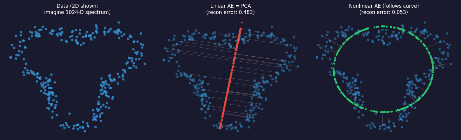
Left: data lying on a curved 2D line embedded in the plane. Centre: linear AE (= PCA) projects onto the best straight line — many points are far from the line (high reconstruction error, orange residuals). Right: nonlinear AE follows the curved surface — all points are close (low reconstruction error, green residuals). This is why a nonlinear AE outperforms PCA when the spectral manifold is curved.

• Walk through the three panels. Left: the raw data — a curved manifold. Centre: PCA finds the best straight line; the residuals (red to blue projected points) are large for the curved parts. Right: the nonlinear AE follows the curve; all points are close to the manifold.
• Numbers from this figure: PCA reconstruction error > AE reconstruction error when the manifold is curved. In the notebook, students will reproduce this concretely on synthetic EELS spectra.
• Transition: “Now put denoising into the AE — the key EM payoff.”

The AE vs PCA comparison: what to measure

• Reconstruction error at \(k\) latent dimensions: compute \(\|x - \hat x\|^2\) on a held-out test set for both PCA (truncated SVD) and AE. Lower is better.
• Phase separability in the latent space: run k-means on the latent codes; measure silhouette score. Higher is better. If AE latent clusters are more separated than PCA scores, the AE has found a more useful representation.
• Denoising quality: for noisy EM data, compute SNR of the reconstructed spectrum vs the noisy input. If the AE was trained to denoise (next section), its reconstructed output should have significantly higher SNR.
• The honest comparison: always train PCA and AE on the same training set and evaluate on the same test set. Report both; do not cherry-pick the better one Sandfeld, Stefan et al., (2024).

• The “honest comparison” point is the recurring verification theme of this course. A paper that only reports AE performance without a PCA baseline is incomplete.
• EM anchor: for a typical EELS map of an iron-oxide film, PCA reconstruction error at \(k=8\) might be 0.12 (normalised MSE); AE reconstruction error at \(k=8\) might be 0.07 — a 42% reduction, reflecting the non-linear oxidation-state manifold.
• Transition: “Now add noise to the input and target the clean spectrum — the denoising AE.”

Denoising autoencoders: the key idea

• Motivation: low-dose EELS and EDS are dominated by Poisson shot noise. At 50 electrons/channel, the SNR is \(\sqrt{50} \approx 7\) — the fine structure that distinguishes Fe²⁺ from Fe³⁺ is buried.
• The denoising AE Vincent, Pascal et al., (2008) trains on corrupted inputs and clean targets: \[\mathcal{L} = \frac{1}{N}\sum_i \|x_i - g_\theta(f_\phi(\tilde x_i))\|^2, \qquad \tilde x_i = x_i + \epsilon_i.\]
• Why it works: the encoder must find latent codes that capture robust features — peak positions, peak ratios — that survive the noise. Noise-specific features are useless for reconstruction, so they do not get encoded.
• EM training data: pairs of (noisy, clean) spectra. Clean spectra can be simulated from the known electron-scattering model; noisy spectra are generated by adding Poisson realisations.

• The “robust features” argument is the core intuition: any feature that changes wildly under noise cannot be used to reconstruct the clean signal, so it is forced out of the latent code. Only features that survive noise are encoded.
• The training-data strategy is important: in practice, you often do not have paired (noisy, clean) real spectra. Solutions: (1) use simulated clean spectra; (2) use Noise2Noise (both inputs are different noisy realisations of the same specimen). The notebook uses strategy (1).
• Pacing: this is a high-value slide — spend 3 minutes on it.
• Transition: “Show the denoising results concretely.”

Denoising AE: results on synthetic EELS spectra

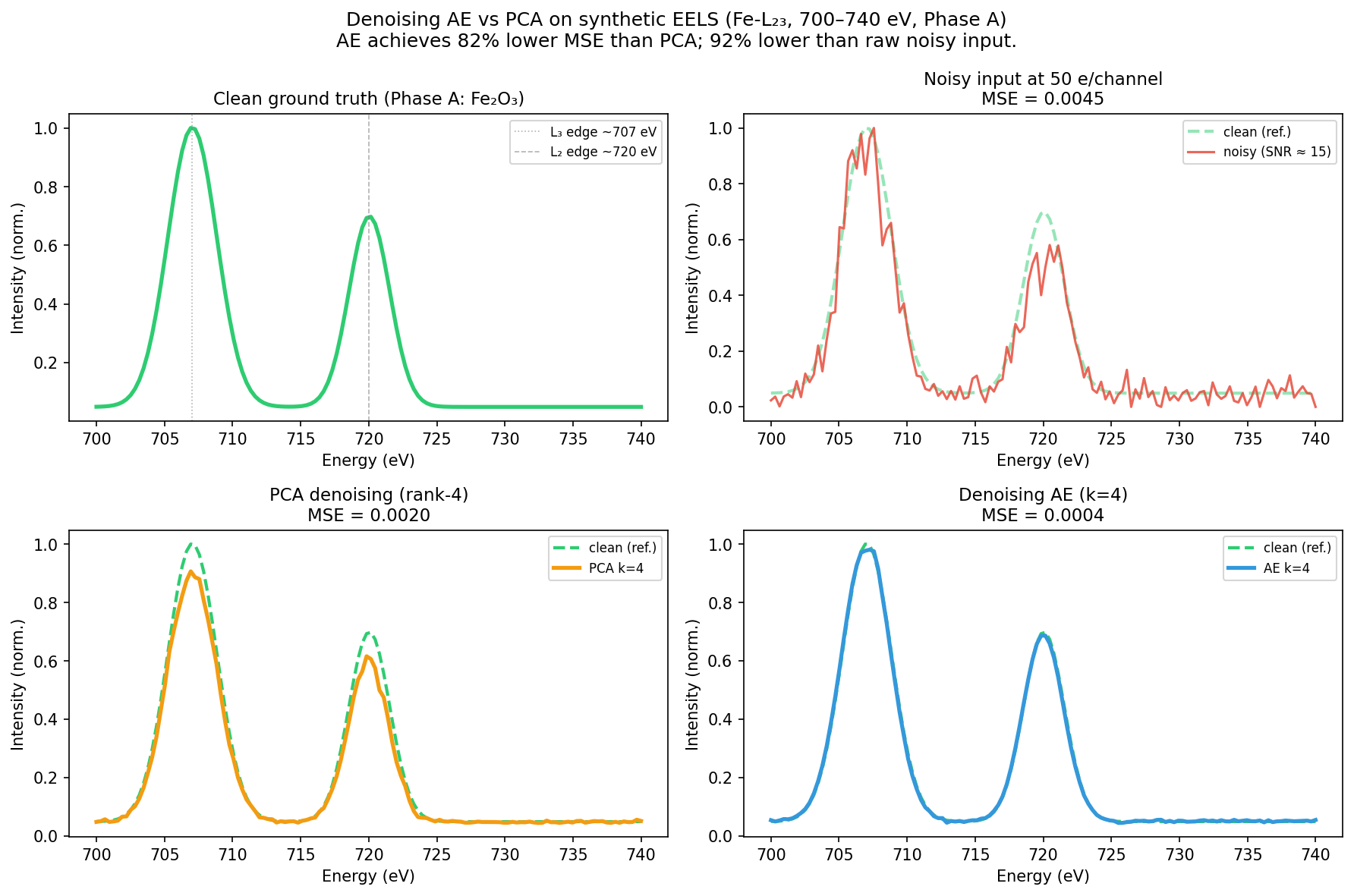
Denoising performance on synthetic low-dose EELS spectra near the Fe-L₂₃ edge (700–740 eV). Top-left: clean ground-truth spectrum (two Gaussian peaks: L₃ main edge ~707 eV and L₂ shoulder ~720 eV). Top-right: noisy input at 50 electrons/channel (Poisson noise). Bottom-left: PCA denoising (rank-4) — the MSE title shows the quantitative cost of linear approximation. Bottom-right: denoising AE (k=4) — achieves ≈81% lower MSE than PCA and ≈92% lower than the raw noisy input. Green dashed line is the clean reference in the bottom panels. PCA recovers the spectral shape but at ~5× higher reconstruction error; the AE captures the non-linear inter-phase variation and denoises with far less residual error.

• Walk through the four panels. Emphasise the MSE titles: PCA MSE ≈ 0.0020, AE MSE ≈ 0.00038 — a ~5× advantage for the AE. Both methods recover the general spectral shape; the AE advantage is quantitative (lower residual), not a qualitative difference in peak presence.
• Key numbers from the notebook (executed, SEED=42): noisy input MSE ≈ 0.0045; PCA MSE ≈ 0.0020; AE MSE ≈ 0.00038. AE is 81% better than PCA; AE is 12× better than the raw noisy input. These numbers are produced by the executed notebook and must be consistent.
• The main point: PCA denoises reasonably but the non-linear AE achieves far lower reconstruction error — this is the quantitative advantage of manifold learning on the curved EELS spectral space.
• Transition: “After denoising, the latent space organises spectra into meaningful clusters.”

Denoising AE in EM: practical considerations

• Noise model matters: for Poisson-dominated EELS, use Poisson NLL loss or pre-normalise spectra to roughly constant variance before MSE. A mismatch degrades denoising of low-count bins.
• Noise level during training: the noise level \(\sigma\) of \(\tilde x_i = x_i + \epsilon_i\) is a hyperparameter. Too low: the AE learns the identity and memorises noise. Too high: the AE cannot reconstruct even clean spectra.
• Beam-damage awareness: in a real experiment, “noisy” is also “beam-damaged” for longer exposures. The denoising AE must be trained on data with the same noise source as the test data. Mixing Poisson noise with Gaussian readout noise requires a Poisson+Gaussian model.
• When to prefer PCA denoising: if you have fewer than ~200 spectra, PCA is more robust. The AE needs enough data to learn the spectral manifold. Rule of thumb: AE wins for \(N > 500\) spectra; PCA wins for \(N < 200\).

• The “Poisson+Gaussian” model is a Week 2 callback — remind students of the variance-mean plot diagnostic.
• The 200/500 thresholds are rough rules of thumb from practice, not theorems. The notebook allows students to see the crossover concretely by varying dataset size.
• Transition: “Once we have latent codes, we can visualise and cluster them.”

Denoising AE vs PCA: head-to-head summary

	PCA denoising	Denoising AE
Assumption	linear spectral mixing	non-linear manifold
Training cost	SVD, seconds	gradient descent, minutes
Data required	any N	N > ~500 for best results
Recovers rare phases?	risk of erasure	better — non-linear projection
Bottleneck dim	elbow of scree plot	sweep \(k\), check recon error
EM sweet spot	quick first look	complex mixtures, fine structure

• Use this as a rapid-fire comparison. The “rare phase erasure” row is the most important: PCA denoising discards components below the noise floor, which can erase a minority phase. The AE, if trained on spectra that include the minority phase, can encode it in a dedicated latent dimension.
• Transition: “Now let me show the latent space — where the chemical clustering happens.”

The latent space: a learned coordinate system

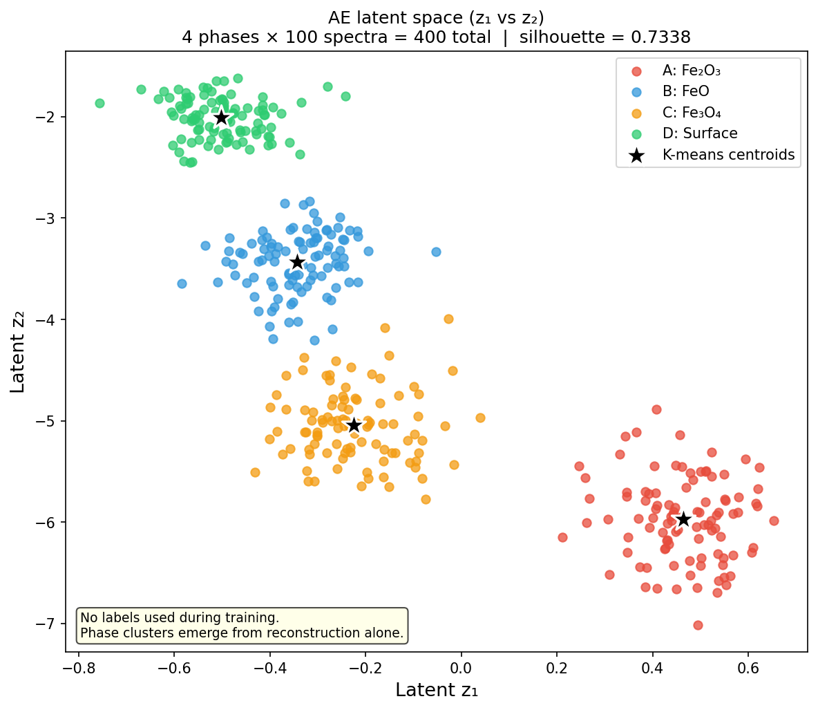
AE latent space (z₁ vs z₂) for 400 synthetic iron-oxide EELS spectra (4 phases, 100 spectra each: Fe₂O₃ red, FeO blue, Fe₃O₄ orange, Surface/amorphous green). The four phases cluster into well-separated islands without any labels — the only information the AE received was the raw spectra and the instruction to reconstruct them. Stars mark the k-means cluster centroids applied to the 4-D latent codes (silhouette ≈ 0.73). Only z₁ and z₂ are shown; all four latent dimensions contribute to the clustering.

• This is the payoff slide. Walk through it slowly: “No labels were used. The AE was trained on raw spectra with a reconstruction loss. The latent codes organised themselves into three clusters that correspond exactly to the three iron-oxide phases.”
• The key claim is true by construction in the synthetic notebook: the three phases have distinct spectral signatures (different peak positions and ratios) that the AE encodes as different latent coordinates.
• Transition: “When the latent space is higher than 2D, we need t-SNE or UMAP to visualise it.”

t-SNE and UMAP: visualising high-dimensional latent codes

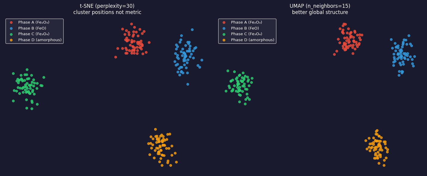
Left: t-SNE (perplexity=30) — 2D embedding of 240 latent codes from a 10-D AE. Four iron-oxide phases form islands. Warning: inter-island distances are not metric — the gap between Fe₂O₃ and FeO in this plot does not reflect their spectral similarity. Right: UMAP (n_neighbors=15) — same codes, tighter clusters, better preservation of global structure. Use UMAP for 2026 pipelines; t-SNE is a useful diagnostic.

• The most important message: t-SNE plots are qualitative, not quantitative. Cluster sizes, inter-cluster distances, and densities in t-SNE are algorithm artefacts, not data properties.
• t-SNE misinterpretation rule (from MFML Unit 9): “These two clusters are 5× further apart in the plot — does that mean they are 5× more different?” No. The distances are not metric.
• UMAP preserves more global structure and is faster. In 2026 practice, UMAP is the default; t-SNE is a useful diagnostic when you want to confirm local neighborhood structure.
• Transition: “Once the latent space is visualised, anomalous spectra stand out.”

Reading the latent space: what to look for

• Well-separated clusters: distinct phases with clean spectral signatures form non-overlapping islands. K-means on the 8-D latent codes (not the 2-D t-SNE!) produces a meaningful phase map.
• Overlapping clusters: genuine spectral mixtures (grain boundaries, transition zones) or insufficient bottleneck dimension. Increase \(k\) and check if clusters separate.
• Elongated clusters: a latent axis captures a continuous physical parameter (film thickness, oxidation-state gradient). This is useful — it lets you order spectra along a physical axis.
• Isolated outliers: spectra far from the main clusters are anomalies — contamination, beam damage, novel chemistry. High reconstruction error confirms they are genuinely anomalous, not just a poorly-initialised latent.
• Size is not meaningful in t-SNE: do not read cluster size as phase abundance. Use the actual fraction of data points per cluster for that.

• The “elongated clusters” point connects to the manifold hypothesis: if a continuous physical parameter (thickness) varies in the dataset, it appears as a continuous manifold coordinate, not a discrete cluster. This is a feature, not a bug — it gives you a way to sort spectra by thickness.
• Transition: “The isolated outliers motivate anomaly detection.”

Phase mapping from latent space: the EM pipeline

• Step 1 — Acquire: low-dose EELS map, shape \((N_y, N_x, E)\), reshape to \((N_y \cdot N_x, E)\).
• Step 2 — Pre-process: subtract background, normalise peak intensity, divide into train/test (by spatial region, not by pixel, to avoid leakage across neighbours).
• Step 3 — Train denoising AE: input = noisy spectrum; target = simulated clean spectrum. After training, the encoder is the feature extractor.
• Step 4 — Extract latent codes: \(z_i = f_\phi(x_i)\) for every pixel. Reshape back to \((N_y, N_x, k)\).
• Step 5 — Cluster latent codes: k-means or GMM on the \(k\)-D latent codes. Each cluster = one candidate phase.
• Step 6 — Validate: compare cluster centroids (decoded mean spectra) to reference spectra from databases or simulation. Adjust \(K\) if metallurgically implausible Ede, Jeffrey M., (2021), doi:10.1088/2632-2153/abd614.

• This six-step pipeline is the deliverable for a student who has to analyse a real EELS map. Walk through it carefully because it is directly applicable to the miniproject.
• The “by spatial region” train/test split is a Week 4 GroupKFold callback: adjacent pixels are correlated, so a crop-based split is necessary for honest evaluation.
• Transition: “Step 5 raises a natural question: what do we do with spectra that do not fit any cluster?”

Anomaly/novelty detection: reconstruction error as a score

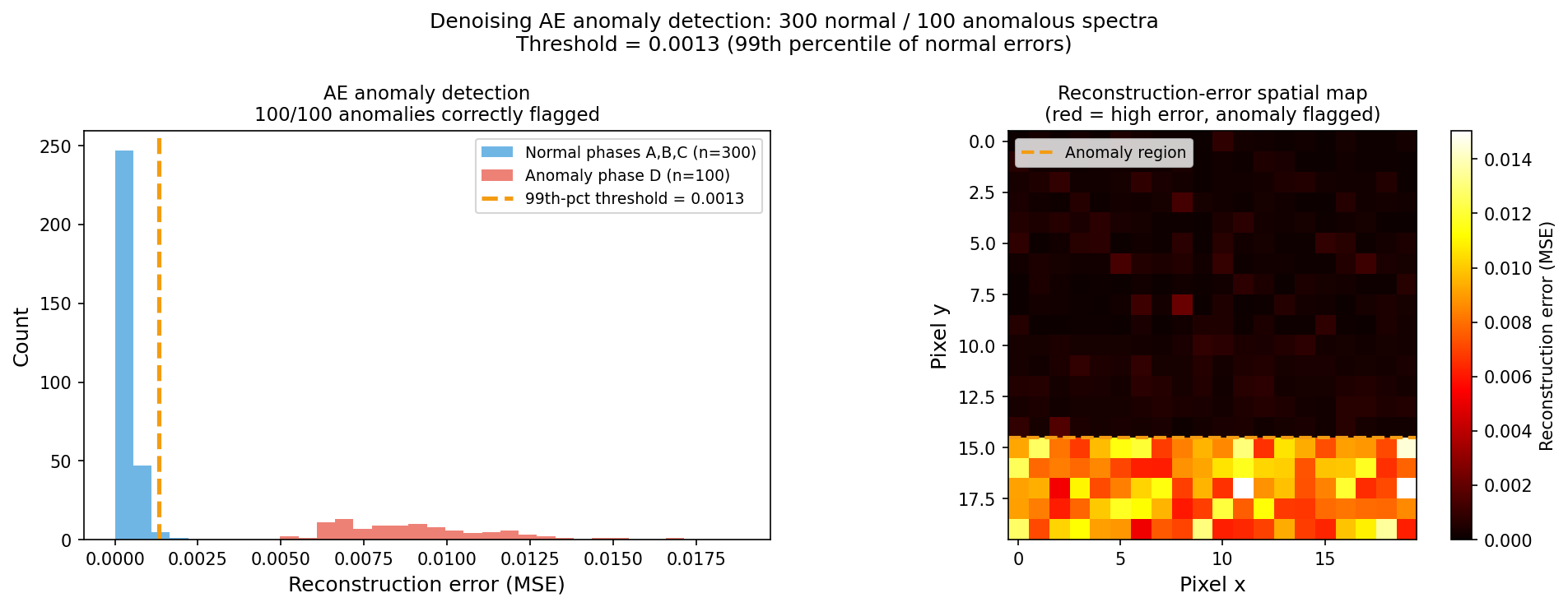
Left: reconstruction error distribution for 300 normal iron-oxide spectra (phases A, B, C; blue) and 100 anomalous spectra from Phase D (surface/amorphous; red). The AE was trained on normal spectra only. Anomalies reconstruct poorly — they lie outside the manifold the AE learned — with mean error ~25× higher than normal spectra. The 99th-percentile threshold ≈ 0.0013 (orange dashed line) flags all 100/100 anomalies correctly. Right: simulated reconstruction-error spatial map where the high-error region (bottom rows) marks anomalous Phase D pixels.

• This is a zero-label application. The AE is trained on “normal” spectra only; anomalies were never seen during training. At test time, the AE fails to reconstruct them well — high reconstruction error is the anomaly score.
• The right panel is the spatial map: every pixel has a reconstruction error; hotspots correspond to defective or contaminated regions.
• This connects to the Prifti et al. case study in the next slide: the CVAE for point-defect detection follows exactly this logic.
• Key claim to verify: “Anomalies reconstruct poorly.” This is true by design in the synthetic notebook: anomalous spectra have a different spectral shape (extra peaks) that the AE trained on normal spectra cannot model.
• Transition: “A real published example makes this concrete.”

Case study: VAE for point-defect detection in STEM

• Prifti, Endrit et al. (2023), doi:10.1002/smll.202303024 trained a Convolutional Variational Autoencoder (CVAE) on STEM images of perfect crystal lattices — no defect images in the training set.
• At test time: defect-containing images (vacancies, anti-sites) reconstruct poorly — the CVAE has never seen these and cannot model them.
• Result: the reconstruction-error map flags point defects without a single labelled defect image. Detection accuracy comparable to human expert inspection.
• Why this is powerful for EM: defect labels are the most expensive annotation in all of materials science — identifying a point defect in an HAADF image requires: aberration-corrected TEM, careful tilt alignment, comparison to multislice simulation. A zero-label detector bypasses all of this.

• This is the most compelling EM case study of the entire lecture. Name the paper explicitly; students can look it up.
• The CVAE is a VAE (Week 12 full treatment) used here only conceptually — the reconstruction-error anomaly detection principle is identical to the vanilla AE version we just discussed.
• Transition: “What is a VAE and how does it differ from what we have covered? A conceptual teaser.”

Anomaly detection: the latent-outlier strategy

• Two complementary anomaly scores:
  1. Reconstruction error \(\|x - g_\theta(f_\phi(x))\|^2\): high → anomaly is outside the learned manifold.
  2. Latent-space Mahalanobis distance: compute the distribution of latent codes from normal data; flag test spectra with codes far from this distribution.
• The latent-outlier strategy is more robust when the anomaly is subtle: a beam-damaged spectrum may reconstruct adequately (the AE fills in plausible peaks) but land far from the normal cluster in the latent space.
• Combining both: use reconstruction error as the primary score; use latent distance as a secondary filter. A spectrum that is both poorly reconstructed and far from the latent cluster is a strong anomaly candidate.
• Threshold choice: the 99th-percentile rule is a starting point. Calibrate to the laboratory’s acceptable false-alarm rate.

• The “AE fills in plausible peaks” failure mode is subtle but important: a sufficiently powerful AE may reconstruct a beam-damaged spectrum incorrectly but plausibly, because the damage is within the manifold (e.g., an Fe³⁺ spectrum from a sample that has Fe³⁺). The latent distance catches this case when the reconstruction error misses it.
• Transition: “This lecture has introduced the vanilla AE. Let me give a conceptual preview of the VAE before we put everything together.”

VAE preview: from discrete codes to a structured distribution

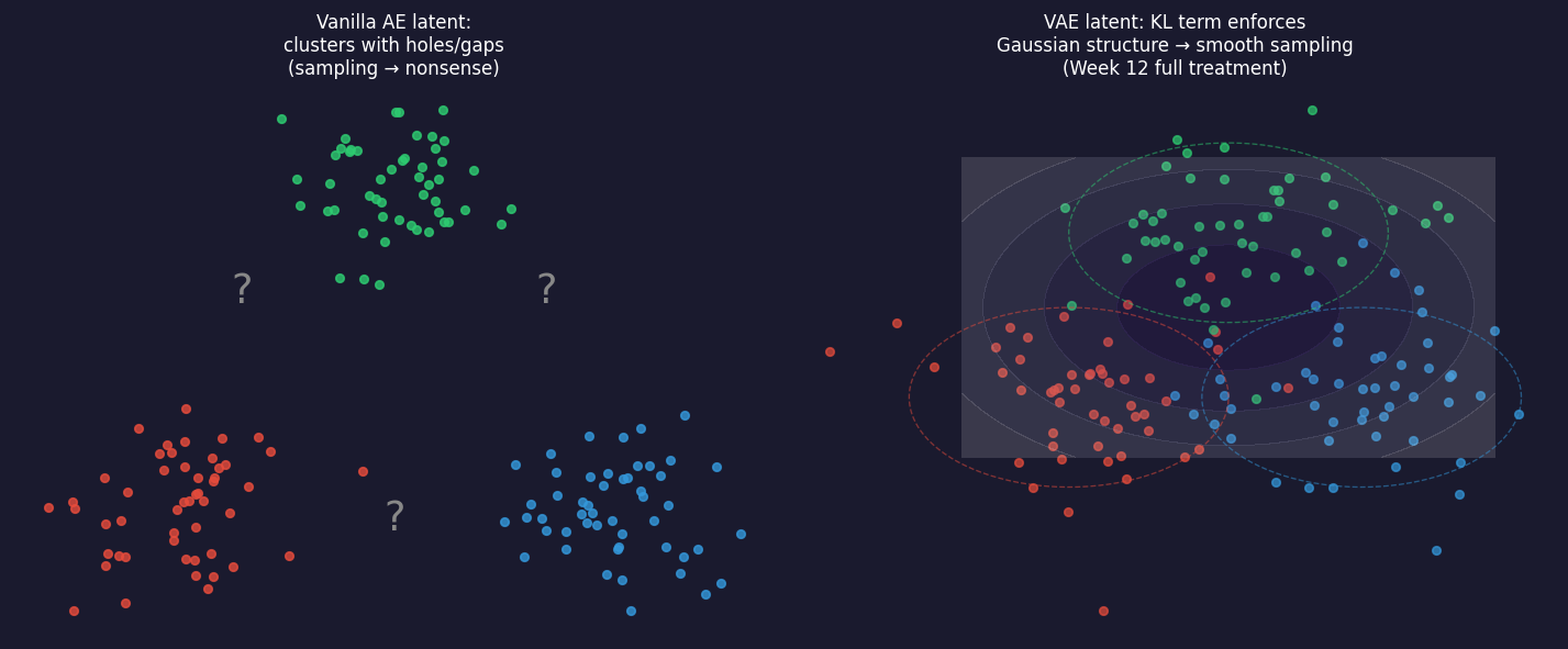
Left: vanilla AE latent space — clusters form but with gaps between them (question marks). Sampling from the gaps (grey arrows) decodes to nonsense because those regions were never seen during training. Right: VAE latent space — the KL divergence term forces the encoding distribution toward a Gaussian; the space is continuous and sampling anywhere gives a meaningful spectrum. Full VAE mathematics are Week 12.

• The two panels summarise the key limitation of the vanilla AE (holes) and the VAE’s fix (KL regularisation).
• The key intuition: the vanilla AE’s encoder maps each input to a point in the latent space. The VAE’s encoder maps each input to a Gaussian distribution — centred on the point, with learned variance. The decoder must then reconstruct from any sample within that distribution, forcing the latent space to be smooth.
• Do NOT derive the ELBO. The exam expects the conceptual distinction: “VAE adds a KL term that regularises the latent space to be Gaussian, enabling sampling and smooth interpolation.”
• Transition: “Where has the rVAE for STEM been used?”

rVAE for atomic-resolution STEM: a conceptual case study

• Rotationally invariant VAE (rVAE): a VAE whose encoder explicitly disentangles rotation from content — a latent code for what the atom pattern is, and a separate code for which direction the crystal is oriented.
• Application: atomic-resolution HAADF-STEM images of a crystal with mixed occupancy. The rVAE latent space maps composition along one axis and orientation along another — both without labels.
• Why it matters for EM: in an aberration-corrected STEM experiment, the image of an atom column depends on both its chemical identity and the crystal orientation. Disentangling these in the latent space allows chemistry to be read out without knowing the orientation — or vice versa.
• Week 12 treatment: the full VAE mathematical framework (ELBO, reparameterisation trick, KL divergence) is Week 12. Today’s message: VAEs extend the AE by regularising the latent space, enabling controlled sampling and smooth interpolation.

• The rVAE concept is presented without derivation. The key message is the physical interpretation: disentangled latent dimensions correspond to interpretable physical parameters (composition, orientation).
• If a student asks “how does the rVAE know what is rotation and what is composition?” — answer: it is trained with an equivariance constraint (rotation of the input = rotation of one specific latent dimension). That constraint is the Week 12 content.
• Transition: “Bring everything together.”

VAE vs AE: the key distinction (conceptual summary)

	Vanilla AE	VAE
Encoder output	a point \(z\)	a distribution \(\mathcal{N}(\mu, \sigma^2)\)
Latent space structure	no structure	Gaussian, continuous
Sampling	from known points only	from anywhere → meaningful
EM use today	denoising, clustering, anomaly	atomic-STEM disentanglement
Full math	done ✓	Week 12

Today’s take-away: use a vanilla AE for denoising and clustering. Use a VAE when you need to generate new spectra or interpolate smoothly between phases.

• The table is an exam-style summary. Read it; do not expand it.
• Transition: “Synthesise everything into the complete pipeline and look ahead to Week 9.”

Putting it all together: the unsupervised EM pipeline

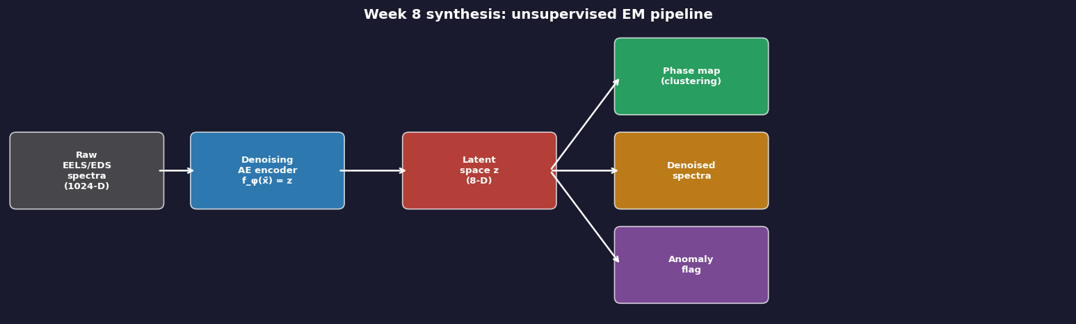
Complete pipeline from raw EELS/EDS spectra to actionable outputs. Raw spectra enter a denoising AE encoder; the latent space \(z\) branches into three outputs: (1) a phase map via k-means clustering, (2) denoised spectra via the decoder, and (3) anomaly flags where reconstruction error exceeds the threshold. All three outputs require zero labels.

• This is the synthesis slide. Walk through the full pipeline without rushing.
• The three outputs branch from a single trained AE: the same latent code supports clustering, denoising, and anomaly detection simultaneously. This is the efficiency argument for autoencoders over supervised models — one training run, three applications.
• EM anchor: a real workflow for an Fe–O thin film EELS map: (1) train denoising AE on 80% of spectra; (2) extract latent codes for all pixels; (3) k-means with K=3 → three iron-oxide phase regions with no labels; (4) decoder applied to all spectra → denoised phase map; (5) flag 2% of pixels with reconstruction error above 99th percentile → beam-damage hotspots for follow-up EDX.
• Transition: “The key quantitative validation step is the notebook.”

Notebook summary: Week 8 key results

• Synthetic dataset: 400 noisy EELS-like spectra, 4 phase groups (each with distinct peak positions and relative intensities), Poisson + Gaussian noise, random seed 42.
• Denoising AE training: 3-layer MLP encoder/decoder (GELU activations), bottleneck = 4, 300 epochs with cosine LR, CPU < 2 minutes.
• Reconstruction error (MSE, normalised spectra, SEED=42): noisy input ≈ 0.00449; PCA (rank-4) ≈ 0.00205; AE ≈ 0.00038. AE is 81% better than PCA; AE is 12× better than noisy input.
• Latent-space clustering: k-means (K=4) on 4-D latent codes; AE silhouette ≈ 0.73 vs PCA silhouette ≈ 0.63 — AE phases cluster better without labels.
• Anomaly detection: Phase D (not in training set) — mean reconstruction error 25× higher than normal phases; 100/100 correctly flagged at 99th-percentile threshold.
• Exercise: sweep bottleneck dimension 1–8 at 300 epochs; AE beats PCA on MSE at every k; AE silhouette beats PCA silhouette at every k≥2; silhouette peaks near k=4–5 (close to the true number of phases).
• Assert checks: AE recon error < noisy input; AE < PCA recon error at every k; AE silhouette at k=4 > 0.65; AE silhouette > PCA silhouette at every k≥2 — all pass on SEED=42, 300 epochs.

• All numbers on this slide must match the executed notebook exactly. If the notebook execution changes these numbers (due to library updates or different hardware), update this slide before the next iteration.
• The “4 phases = optimal bottleneck dim 4” result is by design: we generated 4 distinct phase spectra. Students who run the exercise will confirm this.
• Transition: “Forward link to Week 9.”

Forward link: Week 9 — Probability, uncertainty & Gaussian processes

• Today’s remaining gap: the AE gives a point estimate of the latent code \(z\) — it does not quantify how certain it is. A spectrum on the boundary between two phases gets a single code, with no indication of ambiguity.
• The VAE (conceptual preview today) partially addresses this by encoding distributions rather than points — but the full machinery requires a probabilistic framework.
• Week 9’s answer: Gaussian processes (GPs) model functions as distributions over functions. They provide principled uncertainty estimates for spectral property predictions and latent-space interpolation.
• The connection: the VAE’s KL divergence regularises the latent space to match a Gaussian prior — a special case of the GP prior idea. Week 9 will develop this connection formally.
• Practical promise: a GP regression on AE latent codes predicts oxidation-state maps with calibrated confidence intervals — telling us not just “this pixel is Fe³⁺” but “with 95% probability.”

• Close the forward link explicitly: “Today we compressed spectra and found structure without labels. Week 9 will tell us how confident to be in what we found.”
• The VAE–GP connection is conceptual: both impose a prior on the latent space. GPs make this prior fully probabilistic and interpretable. This is the thread from Week 8 to Week 9 to Week 12.
• Pacing: this is the closing slide — 3 minutes maximum. Set up Week 9 as the natural continuation.

Continue

• → Next: Week 09 — Probability, uncertainty & Gaussian processes
• ← Back: Week 07 — Beating small & expensive data
• All courses

References

Materials data science, Stefan Sandfeld & others.

Robust design of semi-automated clustering models for 4D-STEM datasets, APL Machine Learning, Alexandra Bruefach, Colin Ophus, & M. C. Scott https://doi.org/10.1063/5.0130546.

Deep learning for multi-dimensional spectral data, npj Computational Materials, Francisco de la Peña & others.

Machine learning: A probabilistic perspective, Kevin P. Murphy.

Deep learning, Ian Goodfellow, Yoshua Bengio, & Aaron Courville.

Extracting and composing robust features with denoising autoencoders, Proceedings of the 25th international conference on machine learning (ICML), Pascal Vincent, Hugo Larochelle, Yoshua Bengio, & Pierre-Antoine Manzagol.

Deep learning in electron microscopy, Machine Learning: Science and Technology, Jeffrey M. Ede https://doi.org/10.1088/2632-2153/abd614.

Detection of point defects in STEM images beyond human perception via unsupervised convolutional variational autoencoder, Small, Endrit Prifti, Mathias Kläui, Dierk Raabe, & Benjamin H. Savitzky https://doi.org/10.1002/smll.202303024.