Data Science for Electron Microscopy
Week 9: Probability, uncertainty & Gaussian processes

Prof. Dr. Philipp Pelz

FAU Erlangen-Nürnberg

Institute of Micro- and Nanostructure Research

Recap: Week 8 and today’s question

• Week 8: autoencoders provide point estimates of the latent code \(z\) — they do not say how confident they are. A spectrum on the phase boundary gets a single code with no indication of ambiguity.
• The remaining gap: the AE says “this pixel is at latent point \(z\)” but gives no error bar. If we use that code to guide an experiment or make an engineering decision, we have no way to know when to trust it.
• Today’s answer: probabilistic models. We replace point predictions with distributions over predictions — and we choose our error bars in a principled, honest way.
• Concrete payoff: a Gaussian Process fitted to a handful of expensive EELS measurements gives calibrated ±2σ bands; the band widens exactly where we have no data, telling us where to measure next.
• Forward link to Week 10: that “where should we measure next?” question is active learning — the direct application of today’s uncertainty estimates to automated EM acquisition.

• Open by closing the loop from Week 8: “last week an autoencoder gave us a point in latent space. Today we ask: how confident is that point?” The two weeks are the same arc — representation then uncertainty.
• EM anchor: a phase-boundary pixel on the Fe₂O₃/FeO interface. The AE puts it at some latent code. Is that code Fe₂O₃ or FeO? With what probability? Today gives the machinery to answer that.
• Pacing: 3 minutes maximum. The key phrase to land: “a number without an error bar is not a deliverable — an engineer who ships a design based on ‘450 MPa’ with no ±interval has committed a professional mistake.”
• Transition: “Let me show the roadmap and then the motivating example.”

Road map and self-study

• Road map: recap Week 8 + today’s question (2) · why a point prediction is dangerous for EM decisions (3) · probability as the language of uncertainty (2) · aleatoric vs epistemic uncertainty with EM examples (3) · from MLE/MSE to predicting a distribution (3) · Gaussian processes: prior, sampling & kernel (3) · conditioning on data: posterior mean ± uncertainty band (5) · kernels: RBF, amplitude & hyperparameter learning (3) · GP closed-form posterior, uncertainty balloons & limitations (4) · conformal prediction: model-agnostic coverage guarantee (4) · MC-dropout & deep ensembles as practical UQ (3) · calibration: are the error bars honest? (3) · GP for small expensive EM datasets + forward link + notebook summary (4) — 42 content slides total (within the 40–48 target).
• Self-study: notebooks/week09_gp_uncertainty.ipynb — fit a GP (GaussianProcessRegressor, RBF kernel, CPU, <30 s) to 8 simulated expensive EELS measurements; plot posterior mean ±2σ; observe the band widening away from data; add a measurement and see the local collapse; explore kernel length-scale under/over-smoothing in the exercise.

• Read the roadmap at medium pace. The two anchors to call out: the “uncertainty balloons” intuition (the GP’s killer feature) and the forward link to Week 10’s active learning. Everything else supports those two payoffs.
• One pacing note: this slide is orientation only — 1 minute. Do not read every bullet. Gesture at the structure and move forward.
• Transition: “Start with why a point prediction can be dangerous.”

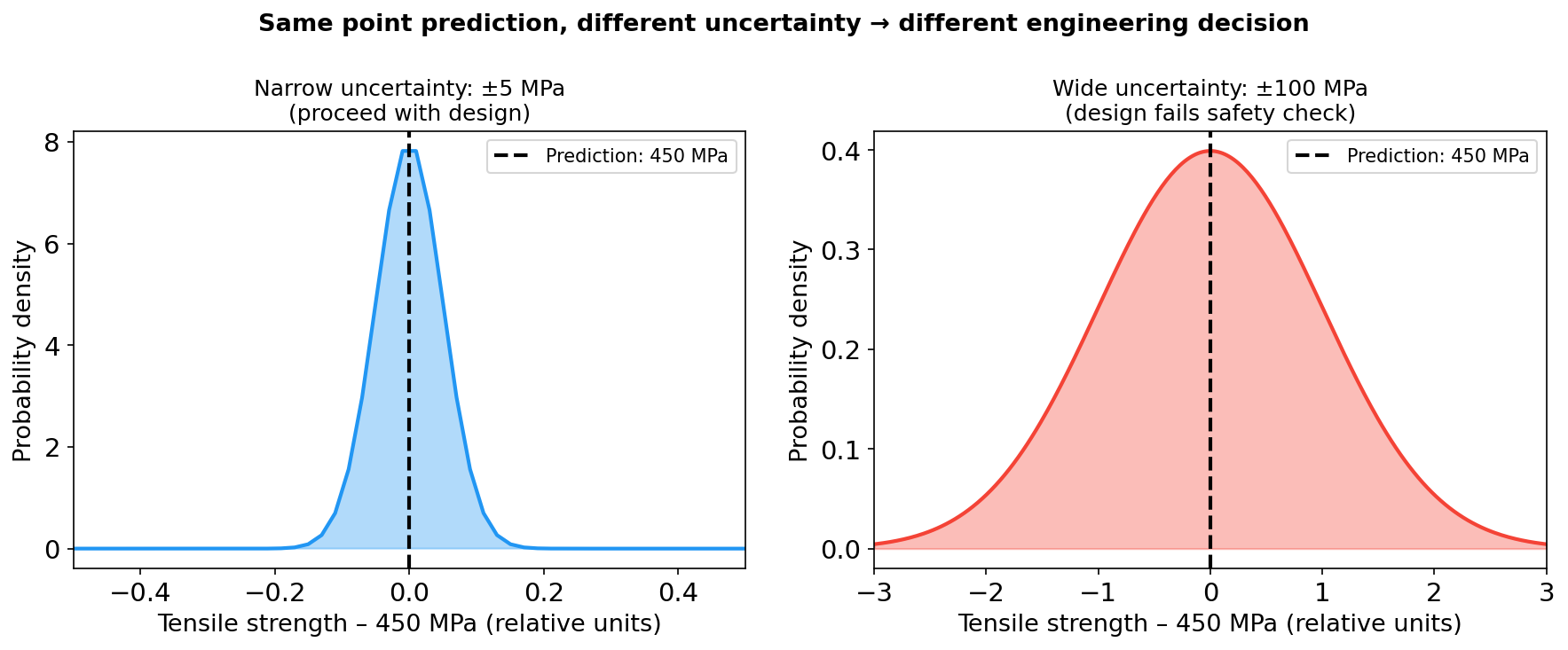
Why a point prediction is dangerous for EM decisions

Two distributions with the same point prediction (450 MPa) but radically different uncertainty. Left: ±5 MPa — the part passes the safety factor. Right: ±100 MPa — the design must be rejected. The engineering decision lives entirely in the uncertainty band, not the mean.

• Walk through the figure: same mean, same label “450 MPa”, completely different consequence. The left model is a yes-decision; the right model is a no-decision. The mean alone cannot make this distinction — the band is the information that matters.
• EM anchor: a GP predicting Fe³⁺ fraction from EELS for a new composition. If the band at the target composition is ±0.02, the measurement is informative. If it is ±0.40, the model is saying “I have no idea” — and the experimenter should measure before deciding.
• The moral: “an overconfident model is more dangerous than an inaccurate one.” Write that sentence and leave it up.
• Transition: “Show two more dangerous consequences of point predictions.”

When point predictions fail in electron microscopy

• Phase identification from a single number: an AE or CNN predicts “Fe₂O₃” for a boundary pixel. Without a confidence score, you cannot know if this is a clean prediction (far from the decision boundary) or a coin-flip. Misidentification propagates silently into phase maps.
• Extrapolation without warning: a model trained on specimens at 200–500 °C predicts properties at 600 °C with the same apparent confidence. The model does not know it is extrapolating. A GP explicitly widens its band in the extrapolation region. Bishop, Christopher M., (2006)
• Expensive experiment design: spending 8 h of instrument time measuring a composition you already know well wastes resources. A model with honest error bars tells you which composition is most uncertain — and is therefore most worth measuring.
• Safety-critical decisions: structural materials for aerospace or energy applications face certification requirements that demand quantified confidence intervals, not point estimates.

• The extrapolation point is the most important. Draw the contrast on the chalkboard: a neural net extrapolates with a smooth, confidently-drawn line extending beyond the data. A GP fans out — its band balloons to the prior width — and explicitly signals “here be ignorance.”
• The four bullets map to four distinct use cases the students will encounter: classification (phase ID), regression (property prediction), active learning (experiment design), and deployment (certification). Each has a different consequence of overconfidence.
• Transition: “To fix this we need a language for uncertainty — probability.”

Overconfident models in EM: a concrete failure mode

• Scenario: a CNN trained on EELS spectra from one Fe–O synthesis route predicts oxidation state for a new route (different precursor, different annealing atmosphere).
• What happens without UQ: the model produces a smooth, confident-looking phase map. Errors are silent — there is no “I don’t know” output.
• What we want: a model that says “for this spectrum (outside my training distribution) I predict 0.6 ± 0.3” rather than “I predict 0.6” — so the experimentalist knows to treat it as a hypothesis, not a measurement.
• Root cause: point-prediction models minimise average error on the training set. They have no incentive to express ignorance. Probabilistic models encode ignorance as wide distributions.

• The “silent failure” phrase is the key. A model that returns NaN is good — you know it failed. A model that returns a confident-sounding wrong number is the dangerous one.
• The training-set-average framing is the technical explanation: MSE measures average accuracy, not calibration. A model that is right 80% of the time but overconfident on the 20% wrong cases has excellent test MSE and terrible practical safety.
• Transition: “We need a mathematical language for this — probability.”

Probability as the language of uncertainty

• Data is noisy. Repeated EELS measurements of the same specimen at the same position give different spectra — photon shot noise, detector readout noise, beam instability. Each is a sample from a distribution.
• Models are uncertain. A regression model fitted to 8 measurements cannot uniquely determine the underlying curve — many curves fit the data. Probability encodes the set of plausible curves.
• Probability provides a rigorous, consistent accounting for both sources of uncertainty simultaneously. The same rules — Bayes’ theorem, the sum rule, the product rule — handle both Bishop, Christopher M., (2006).
• Key shift: instead of asking “what is the true value of \(y\)?” we ask “given the data \(\mathcal{D}\), what is the distribution \(p(y^* \mid x^*, \mathcal{D})\)?”

• “Data is noisy” is the Week 2 callback — they have seen Poisson and Gaussian noise. Now we ask: if every measurement is a noisy draw from a distribution, what does it mean to predict?
• “Models are uncertain” is the key new idea: even if we had a perfect noise model, finite data cannot pin down the model parameters exactly. The parameter uncertainty propagates into prediction uncertainty. This is the epistemic contribution.
• The product rule / Bayes’ theorem angle: tell students that the same mathematical machinery handles both noise and parameter uncertainty. Probability is the unified language.
• Transition: “The distinction between the two sources of uncertainty is the most important concept of today’s lecture.”

From point estimate to predictive distribution

• What MSE training does: find the single parameter vector \(\hat\theta\) that minimises average squared error on training data. Output: one number \(\hat y = f_{\hat\theta}(x^*)\).
• What a Bayesian model does: maintain a distribution over plausible parameter vectors \(p(\theta \mid \mathcal{D})\). Integrate over all of them to get the predictive distribution:

\[p(y^* \mid x^*, \mathcal{D}) = \int p(y^* \mid x^*, \theta)\, p(\theta \mid \mathcal{D})\, d\theta\]

• The predictive distribution is a complete description of our knowledge. Its mean is the best point prediction; its standard deviation is the honest error bar; its full shape encodes the probability of any outcome.
• For a GP this integral has a closed-form solution — exact Bayesian inference with no approximation. Murphy, Kevin P., (2012)

• Read the integral aloud as an English sentence: “for every parameter vector the data finds plausible, ask what it predicts, then average those predictions weighted by how plausible that parameter vector is.” That sentence is the concept; the symbols are bookkeeping.
• The “width comes from parameter uncertainty” framing is the key new idea. The prediction spreads not because the model is noisy — it spreads because many models are consistent with the data, and they disagree. Near data they agree; away from data they disagree.
• The GP closed-form note is the hook for the next major section. Tell them: “in 20 minutes we will see the exact formulas for this integral — two lines of algebra produce the posterior mean and variance.”
• Transition: “Before the GP, we need to clearly separate the two types of uncertainty.”

Aleatoric vs epistemic uncertainty: definitions

• Aleatoric (from Latin alea = dice): irreducible randomness in the data-generating process. The scatter in repeated measurements at the same specimen location — irreducible because it is quantum shot noise. No model, no matter how sophisticated, eliminates it.
• Epistemic (from Greek episteme = knowledge): uncertainty from limited knowledge. We have measured 8 compositions out of infinitely many possible ones. This uncertainty shrinks as we add data.
• The diagnostic test: “Would measuring more of the same kind of data reduce this uncertainty?” Yes → epistemic. No → aleatoric. Bishop, Christopher M., (2006)
• Why it matters for EM decisions: aleatoric uncertainty tells you the achievable precision; epistemic uncertainty tells you where to invest the next instrument-hour.

• The etymologies are memory hooks, not trivia. “Alea iacta est” — the die is cast, irreversible. The shot noise of a photon detector is cast at detection; no averaging removes it from the single measurement. More dose reduces the uncertainty in the mean estimate, but the individual measurement scatter is fixed by physics.
• The diagnostic test is the most examinable concept on the slide. Run through it live with three or four EM examples: grain-to-grain hardness scatter (aleatoric), uncertainty in a hardness model fitted to 5 grains (epistemic), beam-induced carbon deposition drift (epistemic — better vacuum), detector thermal noise (aleatoric).
• The “where to invest” framing is the active-learning hook. A model that clearly separates these two says: “the aleatoric floor is 0.02; epistemic at this composition is 0.15. Measuring here will reduce the total to approximately 0.02.” That is actionable.

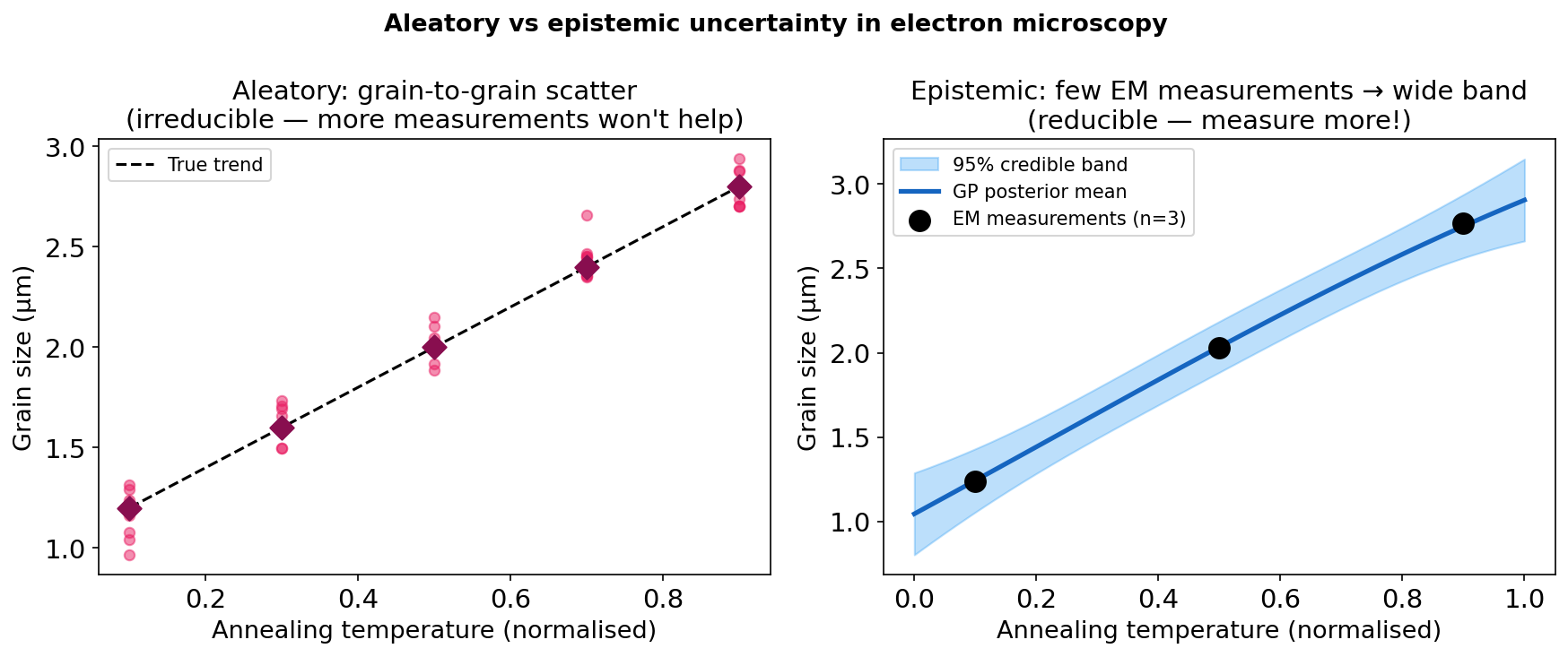
Aleatoric vs epistemic in EM: visual comparison

Left: aleatoric uncertainty — grain-to-grain scatter in grain size measurements at a fixed annealing temperature. More measurements reveal the distribution of grain sizes but do not eliminate the scatter (it is real). Right: epistemic uncertainty — a GP fitted to only 3 EELS measurements (filled circles) is uncertain everywhere except near the measured compositions; measuring more narrows the band. Bishop, Christopher M., (2006)

• Walk through both panels. Left: no matter how many times you measure different grains at the same temperature, you get scatter. The scatter is the data — it describes the material’s real variability. A smaller error bar here means “average of more grains,” not “more precise instrument.”
• Right: the three measured compositions are known (band collapses to zero there). Between and beyond them: honest ignorance. Adding a measurement at any gap would collapse the band locally.
• Ask the room: “which uncertainty shrinks if I measure 10 more grains at the same temperature?” Left. “Which shrinks if I measure 3 more compositions?” Right. Get both answers before moving on.
• Transition: “These two uncertainty types add together in any real system — the GP keeps track of both.”

The variance decomposition: separating aleatoric and epistemic

The total predictive variance separates cleanly Murphy, Kevin P., (2012):

\[ \underbrace{\mathrm{Var}[y^*]}_{\text{total}} = \underbrace{\mathbb{E}_\theta[\sigma_\epsilon^2(\theta)]}_{\text{aleatoric}} + \underbrace{\mathrm{Var}_\theta[\mu(\theta)]}_{\text{epistemic}} \]

• Aleatoric term: average noise variance across all plausible models. Does not shrink with data — it is the irreducible measurement noise floor.
• Epistemic term: how much the predicted mean varies across plausible parameter vectors. Shrinks with more data — as parameter uncertainty decreases, different models agree.
• For a GP this decomposition is exact: the noise kernel \(\sigma_n^2\) is the aleatoric term; the posterior variance formula gives the epistemic term.
• Active learning target: collect data where the epistemic term is largest — that is where a measurement buys the most reduction in total uncertainty.

• Write the decomposition on the chalkboard and label both terms while reading it. Then underline “does not shrink” under the aleatoric term and “shrinks” under the epistemic term. The visual contrast is the memory hook.
• The GP-specific version: the WhiteKernel noise level σ_n² is the aleatoric floor; the \(k(\mathbf{x}^*,\mathbf{x}^*) - \mathbf{k}_*^\top (\mathbf{K}+\sigma_n^2\mathbf{I})^{-1}\mathbf{k}_*\) term is the epistemic part. Both appear automatically from the posterior formula.
• Active learning hook: “maximize the acquisition function at the point where the epistemic term is largest.” This is the maximum-uncertainty criterion for Week 10. Plant it now.
• Transition: “With this vocabulary in hand, let us move from MSE to probabilistic prediction.”

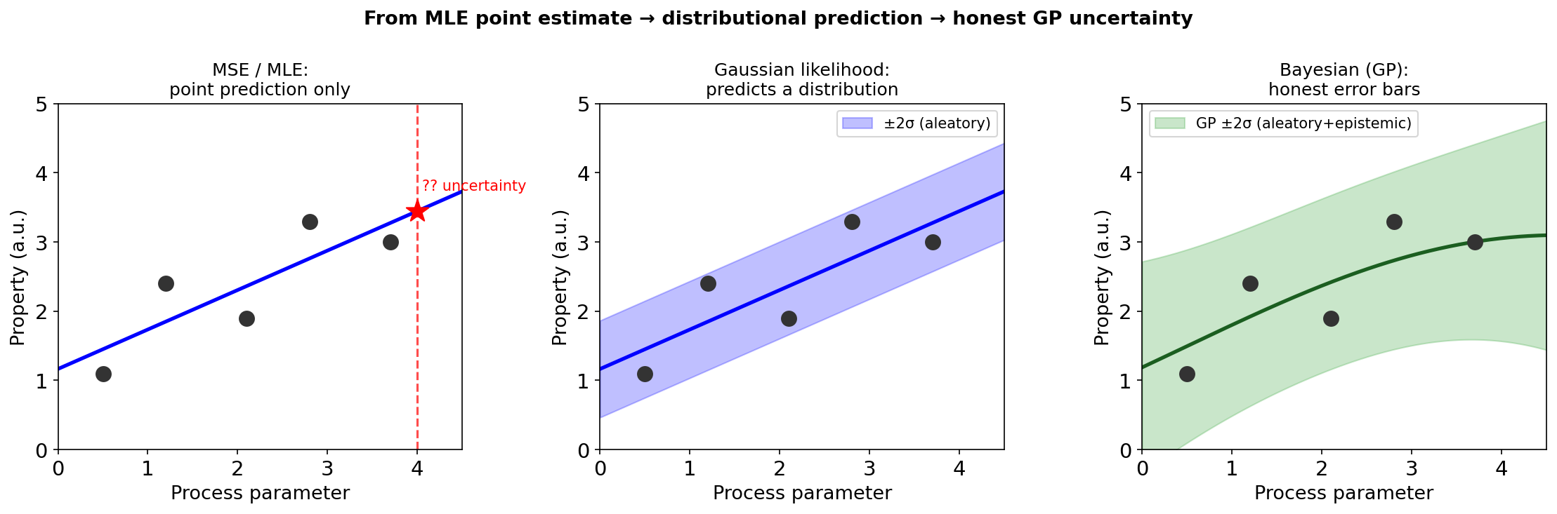
From MLE/MSE to predicting a distribution

Left: MSE regression gives a flat ±σ band everywhere — it models measurement noise, not the model’s uncertainty about the function. Centre: a Gaussian likelihood (Gaussian noise assumed) gives a band but it does not grow away from data. Right: a GP gives a calibrated band that collapses at observations and widens where no data exists.

• Walk through the three panels left to right. Left: the MSE fit. It produces one number per input — a point prediction. If we add the training-residual standard deviation as a constant ±σ, we get a flat band everywhere. It tells us nothing about where the model is confident or uncertain.
• Centre: Gaussian likelihood. Same flat band — the σ is the noise parameter, not a function of how far we are from data.
• Right: GP posterior. The band is a function of x — it collapses exactly at observations, widens in gaps. This is what “honest uncertainty” looks like.
• Ask: “which of these three would you trust for a composition you have never measured?” Right panel, obviously. That intuition is what we make precise with the GP.

Why MSE↔︎Gaussian likelihood and what that implies

• MLE + Gaussian noise = MSE: if we assume \(y = f(x) + \epsilon\) with \(\epsilon \sim \mathcal{N}(0, \sigma^2)\), then maximising the log-likelihood is identical to minimising MSE. This is why MSE is the default loss — it is the correct loss for Gaussian noise.
• What MSE does not give you: the fitted model is a single function \(\hat f\). The uncertainty in the function estimate itself is not captured — MSE treats the function as known once fitted.
• Bayesian extension: instead of a single \(\hat f\), maintain a posterior distribution \(p(f \mid \mathcal{D})\) over plausible functions. The predictive variance then reflects both \(\sigma^2\) (noise) and the uncertainty in which function is correct.
• The GP achieves this exactly by working directly in the space of functions — it is a Bayesian non-parametric model Murphy, Kevin P., (2012).

• The MSE↔︎Gaussian likelihood equivalence is a Unit 4 (Week 4) callback for this course. Students have seen it in regression; now we leverage it as the springboard for the full Bayesian model.
• The key phrase: “MSE is the correct loss but gives you the wrong type of output — a point instead of a distribution.” The GP fixes the type while using the same noise model.
• “Bayesian non-parametric” means the effective complexity grows with data — not that there are no parameters, but that there is no fixed-size parameter vector. The kernel hyperparameters are the “parameters,” but the function is non-parametric.
• Transition: “What is a Gaussian process and why does it give us the distribution over functions we want?”

Fitting a distribution directly: the predictive interval

• The goal: for any new input \(x^*\), produce a distribution \(p(y^* \mid x^*, \mathcal{D})\), not just \(\hat y\).
• The 95% credible interval: \([\mu(x^*) - 2\sigma(x^*),\ \mu(x^*) + 2\sigma(x^*)]\) contains the true value with 95% probability under the model.
• Note on terminology: in Bayesian statistics this is a credible interval, not a confidence interval. The 95% is a statement about our belief given the data, not about the procedure across many datasets.
• Calibration check: a 95% credible interval is calibrated if exactly 95% of test-set observations fall inside it. Miscalibration — too wide (wasteful) or too narrow (dangerous) — is measurable and correctable.

• The credible vs confidence interval distinction is important in practice for defending results in publication. Bayesian credible interval: “I believe the true value is in this range with 95% probability given these data.” Frequentist confidence interval: “95% of intervals constructed this way contain the true value.” Different statements; often numerically similar but conceptually distinct.
• Calibration is the bridge to the end of the lecture: conformal prediction gives a true coverage guarantee; GP credible intervals are calibrated under the model assumptions.
• Plant the calibration theme: “we will come back to ‘are the error bars honest’ in the calibration section. For now, assume the model is correctly specified.”

Gaussian processes: a distribution over functions

• A Gaussian Process is a probability distribution over functions (not over numbers or vectors).
• Formally: any finite collection of function values \([f(x_1), \dots, f(x_n)]\) has a joint multivariate Gaussian distribution:

\[f \sim \mathcal{GP}(m(\mathbf{x}),\ k(\mathbf{x}, \mathbf{x}'))\]

• The GP is fully specified by two functions: the mean function \(m(x) = \mathbb{E}[f(x)]\) (usually 0 after centering) and the kernel function \(k(x,x') = \mathrm{Cov}[f(x), f(x')]\).
• Intuition: drawing a sample from a GP gives an entire curve, not a scalar. The GP is the distribution from which plausible curves are drawn before seeing any data.

• The “distribution over functions” concept is the conceptual leap. Make it concrete: a Gaussian distribution over 2D vectors gives an ellipse of likely (x,y) pairs. A GP over functions gives a “cloud” of likely curves. Each draw from the cloud is one complete function defined at all inputs.
• The multivariate Gaussian restriction: we never work with the infinite object directly. We evaluate it at the finite set of inputs we care about, and those values are jointly Gaussian. This is the trick that makes GPs computationally tractable.
• Zero mean function: “centering” means the GP prior has no a priori trend. After conditioning on data, the posterior mean will be driven by the observations. If you know there is a linear trend, you can put it in \(m(x)\) — the GP then models the residuals.

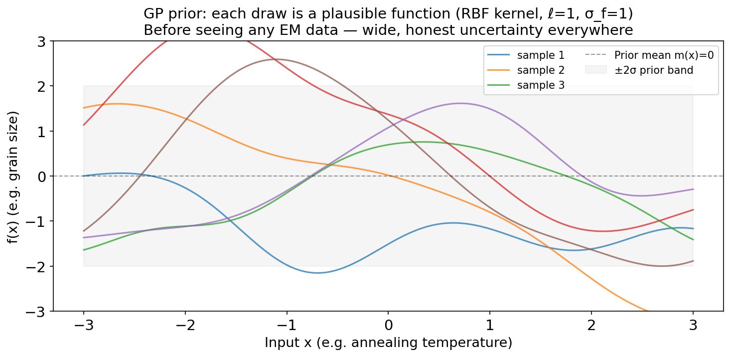
GP prior: drawing plausible functions before seeing data

GP prior with RBF kernel (ℓ=1, σ_f=1). Six random function samples are shown. Before any EM data is observed, the prior expresses equal uncertainty everywhere — no composition is known to be better than any other. Each coloured curve is one plausible ‘model’ of the Fe³⁺ fraction vs composition relationship. The grey band shows the ±2σ prior envelope.

• Walk through the figure slowly. Each coloured curve is one function sampled from the GP prior. They are all smooth (because of the RBF kernel), they all vary on roughly the same scale (amplitude = σ_f = 1), and they all disagree with each other everywhere — because we have not seen any data yet.
• Emphasise: “this cloud of curves is what ‘uncertainty about the function’ looks like.” The width of the cloud at any x is the prior variance σ_f². After conditioning on data, the curves will be forced to pass through (or near) the observations.
• The ±2σ grey band: at every x, 95% of random samples from the prior fall in this band. After conditioning, the band at observed x values will collapse; at unobserved x values it will remain wide.
• Transition: “Now we condition on data — the core GP operation.”

GP prior: what the kernel encodes

• The kernel \(k(x,x')\) is the only part of the GP prior that encodes structure about the function. It answers: “if \(f(x)\) is large, how likely is \(f(x')\) to also be large?”
• The RBF (squared-exponential) kernel:

\[k_\mathrm{RBF}(x,x') = \sigma_f^2\exp\!\left(-\frac{(x-x')^2}{2\ell^2}\right)\]

• This kernel encodes: nearby inputs have correlated outputs, far-away inputs are nearly independent.
• Length-scale \(\ell\): controls the range of correlation. At \(|x-x'| \gg \ell\), \(k \to 0\) — the two outputs are independent. At \(|x-x'| \ll \ell\), \(k \approx \sigma_f^2\) — they are nearly identical. Williams, Christopher K. I. et al., (2006)
• Signal amplitude \(\sigma_f^2\): controls how much the function can vary vertically.

• The kernel is the modelling decision. Choosing a kernel is asserting a belief about the function: “I believe that compositions that differ by less than ℓ have similar Fe³⁺ fractions.” This is domain knowledge encoded mathematically.
• The RBF kernel produces infinitely differentiable (very smooth) functions. Real physical processes might be less smooth — the Matérn-5/2 kernel allows controlled roughness and is often better for materials properties. For today’s intuition, RBF is sufficient.
• Connect the length-scale to the uncertainty band: “at distance ℓ from a data point, the kernel value has dropped to e^{-0.5} ≈ 0.6 — the data point still constrains predictions there. At 3ℓ, the kernel is e^{-4.5} ≈ 0.01 — nearly independent. The band balloons between these regimes.”

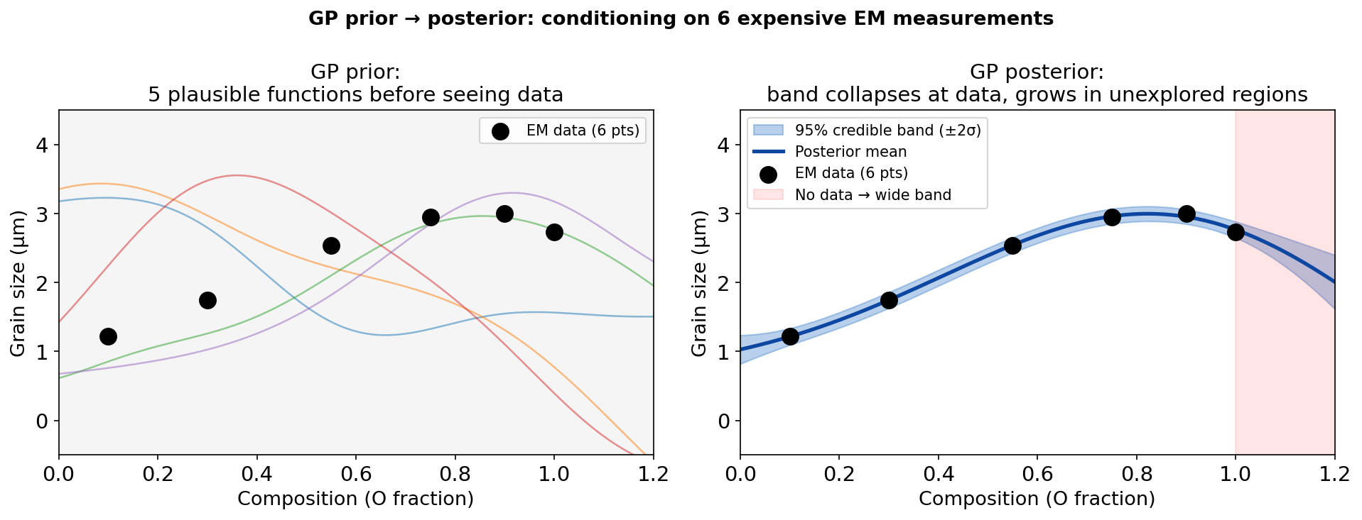
Conditioning on data: GP prior → posterior

Left: GP prior — 5 plausible curves before seeing any EM data. Right: GP posterior after conditioning on 6 EELS measurements (black dots). The posterior curves are forced through (near) the observations; in the unexplored region beyond x=1.0 (red shading) the band widens back toward the prior.

• This is the central pedagogical figure of the lecture. Walk through it carefully.
• Left: the prior cloud. All curves are consistent with “I know nothing about this material system.” Wide uncertainty everywhere.
• Right: the posterior cloud. Every curve now passes near the 6 black dots. The bundle is tight at the data locations and fans out to the right. The key claim: “the GP knows what it doesn’t know — and it says so.”
• Ask the room: “where would the GP tell you to measure next?” Point at the red region. The maximum uncertainty is the maximum information gain — this is the Week 10 hook.
• Transition: “Now show the exact closed-form formulas for the posterior mean and variance.”

GP posterior: how conditioning works (intuition)

• Conditioning a Gaussian on observed values is a standard operation from linear algebra. If \((f, f_\mathrm{obs})\) are jointly Gaussian, then \(f \mid f_\mathrm{obs}\) is also Gaussian — same family, updated parameters.
• The GP exploits this: the joint distribution over \([f(x^*), f(x_1), \dots, f(x_N)]\) is a multivariate Gaussian with mean vector \(\mathbf{0}\) and covariance matrix \([K_{ij}] = k(x_i, x_j)\).
• After observing \(y_i = f(x_i) + \epsilon_i\): the conditional distribution \(f(x^*) \mid \mathbf{y}\) is a Gaussian with updated mean and variance.
• The posterior is another GP. The family is closed under conditioning — no approximation enters here. This is why GPs are called “exact Bayesian” regressors. Williams, Christopher K. I. et al., (2006)

• “Closed under conditioning” is the deep reason GPs are analytically tractable. A Bayesian neural net requires approximate inference; a GP does not. This is the mathematical gift that makes the closed-form formulas possible.
• The jointly Gaussian picture: write the 2-block matrix \(\begin{bmatrix} K_{**} & K_{*N} \\ K_{N*} & K_{NN} \end{bmatrix}\) on the chalkboard. The conditioning formulas are just the conditional-Gaussian formula from linear algebra applied to this block structure. Students who have seen the multivariate Gaussian conditioning formula recognise it immediately.
• Transition: “Here are the two formulas that produce the posterior mean and variance. These are the ones to know.”

GP posterior: conditioning on noisy EM data

• Observe noisy EM data: \(y_i = f(x_i) + \epsilon_i\) with \(\epsilon_i \sim \mathcal{N}(0, \sigma_n^2)\).
• Define the kernel matrix \(\mathbf{K}\) with \([\mathbf{K}]_{ij} = k(x_i, x_j)\) and the cross-vector \(\mathbf{k}_* = [k(x^*, x_1), \dots, k(x^*, x_N)]^\top\).
• The posterior predictive mean at a new input \(x^*\):

\[\mu^*(x^*) = \mathbf{k}_*^\top (\mathbf{K} + \sigma_n^2 \mathbf{I})^{-1} \mathbf{y}\]

• The posterior predictive variance at \(x^*\):

\[\sigma^{*2}(x^*) = k(x^*, x^*) - \mathbf{k}_*^\top (\mathbf{K} + \sigma_n^2 \mathbf{I})^{-1} \mathbf{k}_*\]

These two formulas — closed-form, exact — are all we need for GP regression. Williams, Christopher K. I. et al., (2006)

• These are the two most important formulas in the lecture. Read them aloud as English sentences.
• Mean: “a weighted average of the training outputs, where the weights measure how kernel-similar the query is to each training point.” When x* is near a training point, that point’s y_i dominates the sum. When x* is far from all training data, k_* ≈ 0 and the mean returns to the prior mean (0).
• Variance: “prior variance at x* minus what the data explains away.” The subtracted term is always non-negative — observing data can only reduce variance, never increase it. And crucially: the reduction does not depend on the y values, only on where the data is located. That is the theoretical basis for active learning: knowing where you will measure is enough to plan the reduction in uncertainty.
• The O(N³) cost lives in the matrix inverse. For N=8 (this week’s notebook) this is trivial. For N=10⁴ it is prohibitive — that is the GP’s main limitation.

GP posterior: interpretation in pictures

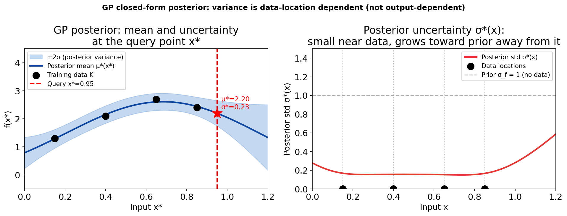
Left: GP posterior mean (blue) and ±2σ band (blue shading) for 4 EELS measurements (black dots). Right: posterior standard deviation σ*(x) as a function of input. The std is near zero at measurement locations and rises toward the prior σ_f=1 in unexplored regions. Observing data can only reduce, never increase, posterior variance.

• Walk through both panels. Left: the full posterior picture we now know how to compute with two formulas. Right: the standard deviation plotted alone — this is the “uncertainty map” for active learning. The two training-data-dense regions show near-zero σ; the gaps and the extrapolation region show high σ.
• The red dashed line on the right panel at σ*=1 is the prior standard deviation σ_f. Notice how the posterior variance approaches but does not quite reach 1.0 even far from data — because the noise kernel (WhiteKernel) also constrains the scale.
• Key exam claim: “GP variance only depends on where data is located, not on what the y values are.” Point at the right panel: there is no information about the y values needed to produce this figure — only the x locations matter. This is a surprising and deeply useful property.

GP posterior: what ±2σ means

• The 95% credible band: for any input \(x^*\), the interval \([\mu^*(x^*) - 2\sigma^*(x^*),\, \mu^*(x^*) + 2\sigma^*(x^*)]\) contains the true function value \(f(x^*)\) with 95% probability under the GP model.
• Narrow band at data: the GP has seen \(y_i \approx f(x_i)\); the posterior constrains \(f(x^*)\) tightly near these locations. Epistemic uncertainty is small there.
• Wide band away from data: as \(x^*\) moves away from all training points, \(\mathbf{k}_* \to \mathbf{0}\); the posterior variance approaches the prior variance \(\sigma_f^2\). The GP reverts to “I don’t know” in the absence of information. Bishop, Christopher M., (2006)
• Honest extrapolation: unlike a neural net that extends a confident line beyond its training range, the GP explicitly widens its band in extrapolation — the most valuable safety property for engineering decisions.

• “95% probability under the GP model” is important to say correctly. The coverage is model-dependent: if the kernel is badly misspecified, the 95% claim may not hold in practice. This motivates the calibration section later.
• “Reverts to the prior” is the physical interpretation: away from data, all we know is what we believed before — the prior. The GP automatically does this with no special casing. It is a consequence of the variance formula: \(\mathbf{k}_* \to 0\) drives the subtracted term to zero.
• Compare to the neural network: a deep net’s output at x far from training data is determined by the last-layer parameters and the activation function. It can confidently extrapolate a sine wave, a line, or a hockey stick — whatever the architecture imposes. There is no honest “I don’t know” built in.

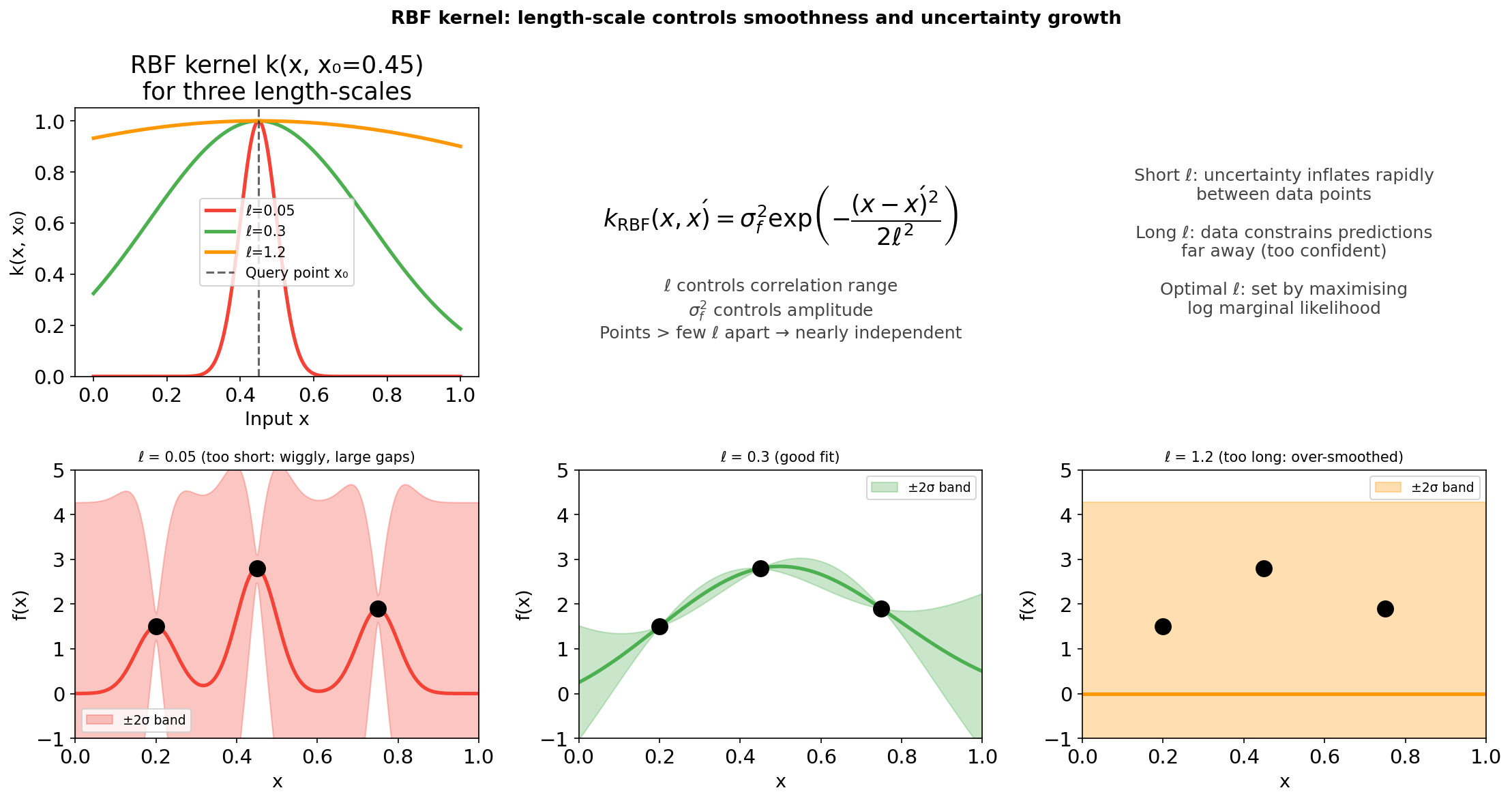
Kernels: RBF and length-scale effects

Top-left: the RBF kernel k(x, x₀=0.45) for three length-scales ℓ. Bottom row: GP posteriors with the same 3 training points but different fixed ℓ. Short ℓ (red): wiggly mean, uncertainty inflates rapidly in every gap. Medium ℓ (green): smooth mean, band widens only in the truly unexplored region. Long ℓ (orange): over-smoothed mean, falsely confident extrapolation.

• Walk through the four panels. Top-left: the kernel shape — as ℓ increases, the kernel stays correlated over longer distances. This directly controls how far a data point “talks to” its neighbors.
• Bottom row left (short ℓ=0.05): uncertainty spikes between every pair of points. The model is honest but useless — it inflates the band in every gap, including the 1-mm gaps between adjacent measurements. Overfitting to local wiggles.
• Bottom row middle (medium ℓ=0.3, the optimised value): smooth mean, band opens only beyond the data range. This is calibrated: confident where data exists, uncertain where it doesn’t.
• Bottom row right (long ℓ=1.2): the mean is oversmoothed and misses the steep S-curve. More dangerously, the band is narrow even far from data — the model is extrapolating confidently, a known failure mode.
• The marginal likelihood is what selects the medium panel automatically. This is the automatic Occam’s razor.

Kernels: amplitude and other kernel families

• Signal amplitude \(\sigma_f^2\): scales the vertical range of function variation. Larger \(\sigma_f^2\) = larger prior uncertainty everywhere. Chosen by maximising the marginal likelihood alongside ℓ.
• Noise level \(\sigma_n^2\): the WhiteKernel. Models measurement noise; allows the GP to pass near observations rather than exactly through them. Separates aleatory (noise) from epistemic (function) uncertainty.
• Matérn kernel (\(\nu=5/2\)): allows less-than-infinitely-smooth functions. More realistic for materials properties that have kinks or discontinuities. Often outperforms RBF in practice.
• Kernel selection: use cross-validation or the log marginal likelihood to compare kernel families. An RBF kernel that is too smooth will underfit a sharp transition; a Matérn-\(\nu=1/2\) (exponential) kernel may overfit kinks. Williams, Christopher K. I. et al., (2006)

• “Maximising the marginal likelihood” is the empirical Bayes procedure: treat ℓ and σ_f as hyperparameters and optimise them. This is what sklearn’s n_restarts_optimizer does — it avoids local optima by running from multiple starting points.
• The Matérn family is the practical default in 2026 GP work: Matérn-5/2 is smooth enough for most physical properties but allows kinks that RBF cannot. If students are fitting real EELS data, recommend Matérn-5/2 over RBF unless they have specific reason to expect infinitely smooth behaviour.
• Kernel combinations: sum = superposition of two behaviours (long-range trend + short-range wiggle). Product = multiplicative interaction. The classic CO₂ seasonal model is RBF × Periodic — a decaying seasonal pattern. This is how GPs can model complex materials signals.

Hyperparameter learning: the log marginal likelihood

• We need to choose \(\ell\), \(\sigma_f\), \(\sigma_n\). Too small ℓ: wiggly and overfit. Too large ℓ: smooth and overconfident. Right ℓ: honest error bars. Murphy, Kevin P., (2012)
• Automatic selection via log marginal likelihood:

\[\log p(\mathbf{y} \mid \mathbf{X}) = -\frac{1}{2}\mathbf{y}^\top(\mathbf{K}+\sigma_n^2\mathbf{I})^{-1}\mathbf{y} - \frac{1}{2}\log|\mathbf{K}+\sigma_n^2\mathbf{I}| - \frac{N}{2}\log 2\pi\]

• The three terms penalise: data misfit (first), over-flexible kernel (second), and a normalisation constant (third). This is automatic Occam’s razor — no separate penalty term needed. Bishop, Christopher M., (2006)
• In sklearn: GaussianProcessRegressor(n_restarts_optimizer=10) maximises this objective from multiple starts. After fitting, inspect gpr.kernel_ for the selected hyperparameters.

• Connect the marginal likelihood to the evidence block from the MFML lectures: “the evidence integrates the likelihood over all parameter values, penalising complexity. Here, the kernel hyperparameters are the ‘hyperparameters’ and the function is the ‘parameters’ — the marginal likelihood already integrates over the function, leaving only the kernel parameters to optimise.”
• The “automatic Occam’s razor” phrase is the key takeaway: the second term (\(-\frac{1}{2}\log|\mathbf{K}+\sigma_n^2\mathbf{I}|\)) penalises a kernel that is too flexible. A short length-scale gives a rich, flexible kernel — the determinant of K grows — and the log-determinant penalty is large. Complexity is paid for automatically.
• Practical note: the marginal likelihood surface can be multimodal. A short ℓ local optimum (wiggly, fits noise) and a long ℓ local optimum (smooth, misses detail) can both exist. The n_restarts_optimizer parameter in sklearn tries multiple starting points to find the global optimum.

GP closed-form posterior: two formulas to know

The GP posterior at new input \(x^*\), given training data \(\mathbf{X}, \mathbf{y}\) and noise \(\sigma_n^2\):

\[\boxed{\mu^*(x^*) = \mathbf{k}_*^\top (\mathbf{K} + \sigma_n^2 \mathbf{I})^{-1} \mathbf{y}}\]

\[\boxed{\sigma^{*2}(x^*) = k(x^*, x^*) - \mathbf{k}_*^\top (\mathbf{K} + \sigma_n^2 \mathbf{I})^{-1} \mathbf{k}_*}\]

• \(\mathbf{K} \in \mathbb{R}^{N\times N}\): kernel matrix \(K_{ij} = k(x_i, x_j)\). \(\mathbf{k}_* \in \mathbb{R}^N\): \([\mathbf{k}_*]_i = k(x^*, x_i)\). Training cost: \(O(N^3)\) for the matrix inversion.
• Mean: weighted average of training outputs; weights proportional to kernel similarity to \(x^*\).
• Variance: prior variance minus the reduction from data. Always \(\geq 0\). Approaches \(k(x^*,x^*)=\sigma_f^2\) as \(x^*\) moves away from all training points.

• These two boxes are the highest-yield formulas in this lecture. Tell students to photograph this slide; they will be asked to reproduce them.
• Mean, physically: “a weighted vote of the training labels. Close training points vote strongly (large k*_i); far training points barely vote (k*_i ≈ 0). If x* is equidistant from two training points with different y values, the mean is their average.”
• Variance, physically: “the prior uncertainty minus what the data explains. The subtracted term is the variance explained by the N training observations. Far from all data, the subtracted term → 0 and σ²* → σ_f². Near a cluster of data, the subtracted term → σ_f² and σ²* → 0.”
• Point at σ_n²I: this is the noise regulariser. Without it (σ_n²=0) the GP interpolates exactly through every training point. With it, the GP passes near but not through each point — the posterior mean is a smoother version of the data.

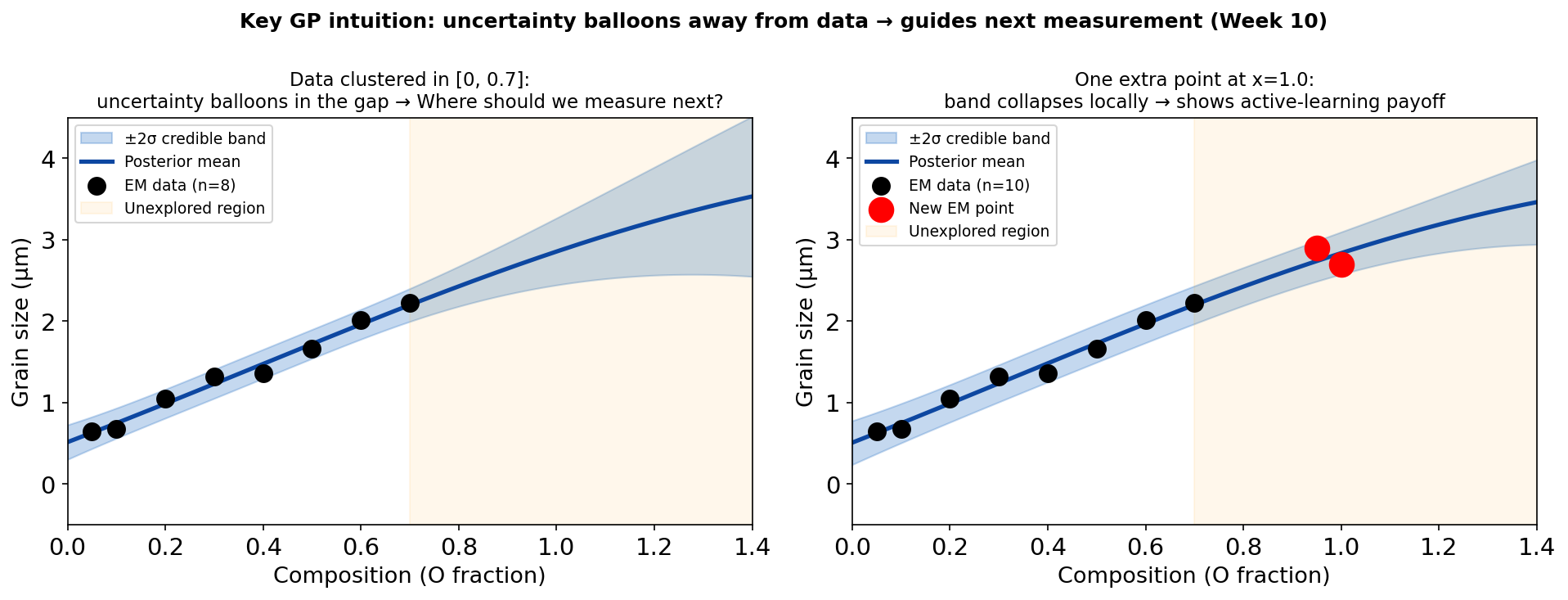
The key intuition: uncertainty balloons away from data

Illustration (generic “grain size vs parameter” example — not the EELS notebook run). Left: GP fitted to 8 measurements with the training cluster in [0,0.7] (as shown on the y-axis). The 95% credible band widens rapidly beyond the data range (red shading) — the GP honestly admits it has no information there. The highest-uncertainty regions are the best candidates for the next measurement. Right: after adding one measurement at x=1.0, the local band collapses (~49% reduction in σ* there) while regions further away remain uncertain. (The EELS notebook uses a cluster in [0.05,0.85] with specific σ* values of 0.1966→0.1003 at x_far=1.15; see the Notebook Summary slide for those numbers.)

• This figure is the emotional payoff of the entire GP block. Let it land.
• Important framing note: this figure is a generic illustration of the balloon concept, with grain size as the y-axis label and training data clustered in [0,0.7] as shown. It is NOT a direct plot of the EELS notebook run (which uses a cluster in [0.05,0.85] and specific numeric values — see the Notebook Summary slide). The figure and caption are intentionally generic so the intuition transfers to any EM dataset; the EELS-specific numbers are discussed separately.
• Left panel: “This is what we built everything for. The blue band is the honest error bar. It is narrow at the 8 black dots — the GP knows what happened there. In the red region it has never been told anything — and it says so by ballooning to the prior width.”
• Right panel: “We simulated what happens when a scientist runs one more experiment at x=1.0. The band at x=1.0 collapses. The band at x=1.15 is reduced but still substantial — one measurement helps but does not eliminate uncertainty. The band at x=0.5 (deep inside the training cluster) is essentially unchanged — far-away data does not help near-data regions much.”
• The ~49% reduction quoted in the caption refers to the generic figure’s proportional change; the notebook-verified numbers (σ* 0.1966→0.1003 at x_far=1.15 in the EELS run) are on the Notebook Summary slide.
• Transition: “This is Week 10’s active learning algorithm in its simplest form: always measure where σ* is largest. We will develop it fully next week.”

GP uncertainty balloons: the formal argument

• As \(x^* \to \infty\) (far from all training data), the kernel vectors \(\mathbf{k}_* \to \mathbf{0}\).
• The variance formula becomes: \(\sigma^{*2}(x^*) = k(x^*,x^*) - \mathbf{0}^\top(\ldots)^{-1}\mathbf{0} = k(x^*,x^*) = \sigma_f^2\).
• The GP reverts to its prior variance — the maximum uncertainty it can express.
• This is an exact result from the posterior formula, not a heuristic. No special code or case-handling needed — it falls out of the math automatically.
• Contrast with neural nets: a neural net extrapolates the function’s value using its learned parameters. It does not widen its band. A GP extrapolates its prior uncertainty — the band expands to the prior width.

• This is the formal version of the intuition from the previous slide. It takes 30 seconds to read through and gives students the algebraic hook: as k_* → 0, the subtracted term vanishes, leaving σ²*.
• The contrast with neural nets is the key practical point for this course. When students run a CNN on new specimen conditions, they get a confident-looking output. When they run a GP on new compositions, they get an honest “I don’t know” band. Neither model is better per se — the GP is better for honest uncertainty, the CNN is better for high-dimensional inputs.
• For active learning (Week 10): the acquisition function max_x σ(x) finds exactly this balloon region automatically. The algorithm does not need to know where “far from data” is — the GP computes σ everywhere and the argmax finds it.

GP limitations: the honest scorecard

	Gaussian Process	Deep Neural Network
Uncertainty	Exact Bayesian, calibrated	Not built-in (requires add-ons)
Training cost	\(O(N^3)\) — limits to \(N \lesssim 10^3\)	\(O(N)\) — scales to millions
Input dimension	Scales poorly beyond ~20-D	Handles 1000-D images natively
Kernel choice	Requires domain knowledge	Learns features automatically
Interpretability	ℓ, σ_f, σ_n are physically meaningful	Weights are uninterpretable
Best use case	Small expensive datasets, tabular	Large datasets, images, sequences

• Use this table as the honest scorecard that closes the GP block. The GP is not universally better — it is specifically better for the regime most common in experimental materials science: small N, tabular inputs, need for calibrated intervals.
• The O(N³) is the single most important limitation. For N=8 (this notebook) it is trivial. For N=1000 it is seconds. For N=10,000 it is minutes. For N=10⁶ it is not feasible — that is the domain of sparse GP approximations, which are out of scope.
• “Learns features automatically” for the DNN is the flip side: a GP with an RBF kernel assumes every input variable is relevant and equally correlated. A DNN can discover that input variable 14 is what actually matters. For 2D inputs (EELS composition maps), the GP is fine. For 100-D descriptor vectors, the DNN is better.

Conformal prediction: model-agnostic coverage guarantee

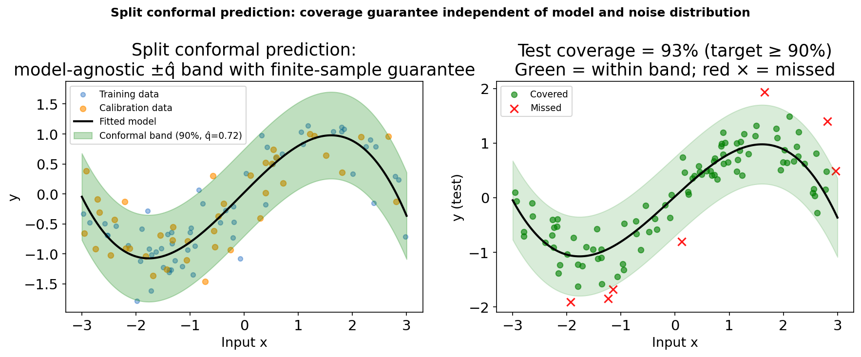
• Problem: a GP’s 95% credible band is calibrated under the model. If the kernel is wrong (misspecified), coverage can be lower. We want a guarantee that holds without the model being correct.
• Split conformal prediction provides a finite-sample, distribution-free coverage guarantee Angelopoulos, Anastasios N. et al., (2023):
  1. Split the data: training set + calibration set.
  2. Fit any predictor on the training set.
  3. Compute residuals \(|y_i - \hat y_i|\) on the calibration set.
  4. Set \(\hat q = (1-\alpha)(1 + 1/n_\text{cal})\)-quantile of calibration residuals.
  5. Output the interval \([\hat y(x^*) - \hat q,\, \hat y(x^*) + \hat q]\) for any new \(x^*\).
• Coverage guarantee: \(\Pr(y^* \in C(x^*)) \geq 1 - \alpha\), for any exchangeable data distribution, any predictor. Angelopoulos, Anastasios N. et al., (2023)

• The “any predictor” is the key selling point. Conformal prediction does not care if the model is a GP, a neural network, or a random forest. It just needs a calibration set and a residual score. The coverage guarantee is distribution-free — no Gaussian assumption, no correct kernel assumption.
• Exchangeability is the one assumption. It means the calibration and test data are drawn from the same distribution — no distribution shift between calibration and deployment. For EM experiments that is usually satisfied (same microscope, same sample type). If there is distribution shift, conformal still adapts — but the guarantee weakens.
• “Split” is the key word: the calibration set is never seen during fitting. It is the held-out set used to calibrate the interval width. This is an extra data split beyond the train/test split of Week 4.
• Transition: “Show the conformal procedure visually.”

Conformal prediction: visual demonstration

Split conformal procedure. Left: the fitted model (polynomial, deliberately underfit) with ±q̂ band (green). The band width q̂ is computed from calibration-set residuals (orange), not from the model’s own uncertainty estimate. Right: test-set coverage = 93% (target ≥ 90%). Green dots = covered; red × = missed. The conformal guarantee holds regardless of model quality.

• Walk through both panels. Left: the model (polynomial) is deliberately underfit — its training residuals are large. Conformal takes those large residuals and sets q̂ to accommodate them. The band is constant-width (split conformal always gives constant width; conformalized quantile regression can give adaptive width).
• Right: 93% of test points fall inside the band — above the 90% target. This is the guarantee working. It doesn’t matter that the model itself is a poor fit; the calibration-set quantile absorbed the model’s errors.
• The red ×: 7% of points fall outside. The guarantee is ≥ 90%, not exactly 90%. The 3% excess is random and would average to exactly 10% over many test sets.
• Important caveat to mention: the constant-width band is the limitation. A GP’s band is narrow near data and wide in gaps — more informative. Conformal’s constant-width band treats all input locations equally. Conformalized Quantile Regression (CQR) gives adaptive-width conformal intervals, combining both advantages.

Conformal vs GP: when to use each

• Conformal strengths: model-agnostic — wraps any predictor. Finite-sample coverage guarantee without distributional assumptions. Easy to implement (one quantile computation). Ideal for deploying any trained model with a certified error bar.
• GP strengths: principled uncertainty that varies with input location (wide gaps → wide band). Interpretable hyperparameters. Enables active learning (measure where σ* is largest). Better for exploration.
• Combined use: fit a GP for uncertainty-guided exploration. Apply split conformal to certify the deployed model’s predictions for safety-critical decisions.
• Common mistake: using training-set residuals instead of calibration-set residuals for the conformal quantile. This breaks the coverage guarantee. Always use a held-out calibration set.

• The “combined use” pattern is the practical recommendation for materials science deployment: GP during the research phase (active learning, exploration), conformal wrapping the production model (certified predictions for a certification body or lab manager).
• The common mistake note is worth making explicit. Students will try to save data by computing q̂ from the training set. This gives optimistically small intervals (the model fits training well) and coverage below the nominal level. The calibration set must be genuinely held out.
• Transition: “Conformal is a wrapper — it requires a trained model underneath. What if the underlying model is a deep neural network?”

Conformal prediction: key properties

Property	Split Conformal	GP Credible Band
Coverage guarantee	Finite-sample, distribution-free	Asymptotic, model-dependent
Band width	Constant (per \(x^*\))	Varies with distance from data
Model required	Any trained predictor	GP posterior
Active learning	Not directly	Natural (maximise σ*)
Computationally	Trivial (sort residuals)	\(O(N^3)\) inversion

Rule of thumb: use conformal to certify; use GP to explore. Angelopoulos, Anastasios N. et al., (2023)

• Table is for rapid orientation. The most important row: “Coverage guarantee.” Conformal: genuine finite-sample. GP: only correct if the kernel is correct.
• The “active learning: not directly” for conformal is a key limitation. Conformal gives you a band at a new point, but the band does not tell you whether measuring there would reduce future uncertainty — it only certifies the current prediction. The GP’s σ* tells you both: current uncertainty AND the potential reduction from measuring.

MC-dropout: uncertainty from a single trained network

• Standard dropout (training only): randomly zero out neurons with probability \(p\). Prevents co-adaptation, reduces overfitting.
• MC Dropout Gal, Yarin et al., (2016): keep dropout active at inference. Run \(T\) stochastic forward passes through the same network. Each pass uses a different random mask → \(T\) different predictions.
• Mean of \(T\) passes: best prediction. Variance of \(T\) passes: approximate epistemic uncertainty.
• Cost: \(T\) forward passes at test time. Zero additional training cost — uncertainty is free from an already-trained network.
• For EM: a U-Net trained with dropout for phase segmentation; at inference, \(T=30\) passes give a per-pixel confidence map. High variance pixels are on phase boundaries.

• The “one line change” hook: standard inference calls model.eval() which disables dropout. MC Dropout calls model.train() (keeping dropout on) at inference. That one line gives approximate Bayesian uncertainty from any network trained with dropout. Tell students this — it is a memorable practical fact.
• The Gal & Ghahramani 2016 theoretical connection: dropout at test time is mathematically equivalent to variational inference in a Bayesian neural net with a Bernoulli approximate posterior. This makes MC Dropout not just a heuristic but a principled approximation.
• The EM application: U-Net for phase segmentation. A deterministic U-Net says “this pixel is Fe₂O₃” with no confidence. An MC Dropout U-Net (30 passes) gives 80% Fe₂O₃, 20% FeO — especially informative at grain boundaries where the phases blend.
• Honest caveat: the dropout rate p must be tuned. Too low: overconfident (interval width ~ 0). Too high: too wide (all pixels look uncertain). The calibration section below shows how to check.

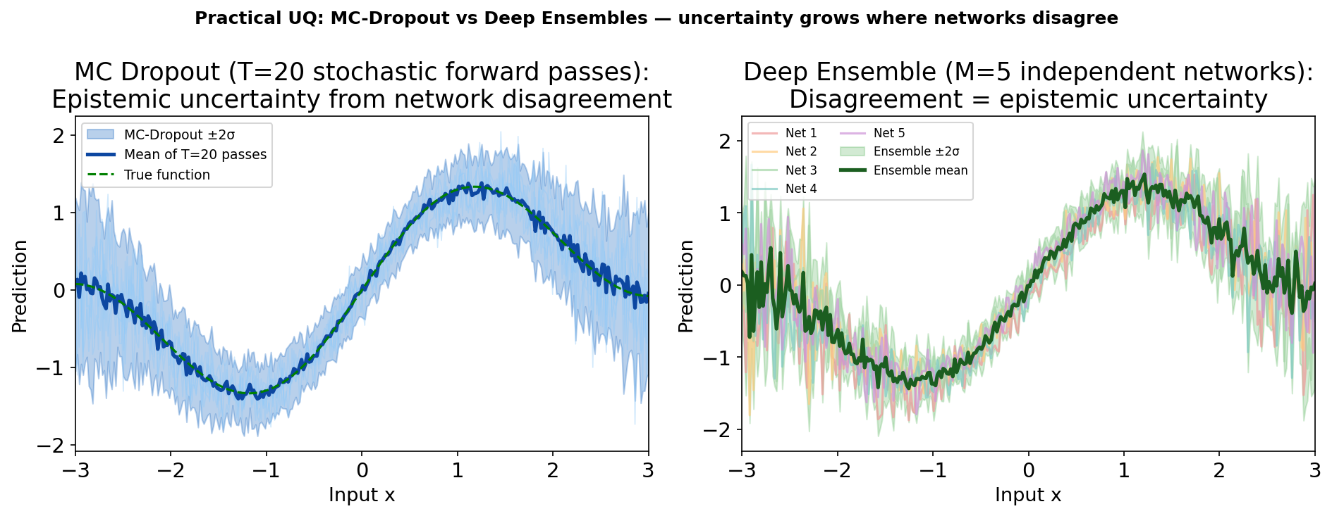
Deep ensembles: best practical UQ for neural networks

Left: MC Dropout — 5 stochastic forward passes (light blue) and the mean ±2σ band. The band widens reasonably away from data but can be sensitive to the dropout rate. Right: Deep ensemble of 5 independently trained networks (different random initialisations and data shuffles). Each network is one coloured curve; the green band is mean ±2σ. Ensembles are empirically the best-calibrated NN uncertainty method Lakshminarayanan, Balaji et al., (2017).

• Walk through both panels. Left: the MC Dropout curves all use the same network weights (same loss landscape) but different masks. The variance reflects the Bayesian posterior approximation.
• Right: the ensemble curves come from 5 entirely different training runs — different random seeds, different mini-batch orderings, different local optima in the loss landscape. Their disagreement IS the epistemic uncertainty, without any Bayesian formalism.
• The Lakshminarayanan 2017 paper result: deep ensembles consistently outperform MC Dropout and many other approximate Bayesian methods on calibration benchmarks. The reason is that different random inits explore genuinely different regions of the loss landscape — true diversity.
• Cost comparison: MC Dropout = T forward passes at inference, zero extra training. Deep ensemble = M full training runs (5× compute) but 1× inference. For a deployed production system, M training runs are done once; inference is cheap.

MC-dropout vs deep ensembles: comparison

	MC Dropout	Deep Ensembles
Training cost	1× (same as baseline)	M× (M full training runs)
Inference cost	T forward passes	M forward passes
Calibration quality	Approximate, sensitive to dropout rate	Best empirical calibration Lakshminarayanan, Balaji et al., (2017)
Diversity	Same local optimum (dropout masks)	M distinct local optima
EM application	Per-pixel uncertainty in segmentation	High-stakes property regression
Theoretical basis	Approximate VI via dropout	Ensemble disagreement (frequentist)

Rule of thumb: MC Dropout if a single trained network already exists and compute is tight. Deep ensemble if budget allows and calibration quality is critical.

• This table is an exam-style summary. The key row: calibration quality. Deep ensembles win by a substantial margin on most benchmarks.
• The “M distinct local optima” point is the theoretical explanation for why ensembles work: the loss landscape of a deep net is non-convex with many local optima. Different random initialisations find different optima, and they disagree where the data is sparse. That disagreement is the epistemic signal.
• For the exam: students should know (1) how each method works in one sentence, (2) the training cost comparison, and (3) the calibration comparison. Everything else is detail.

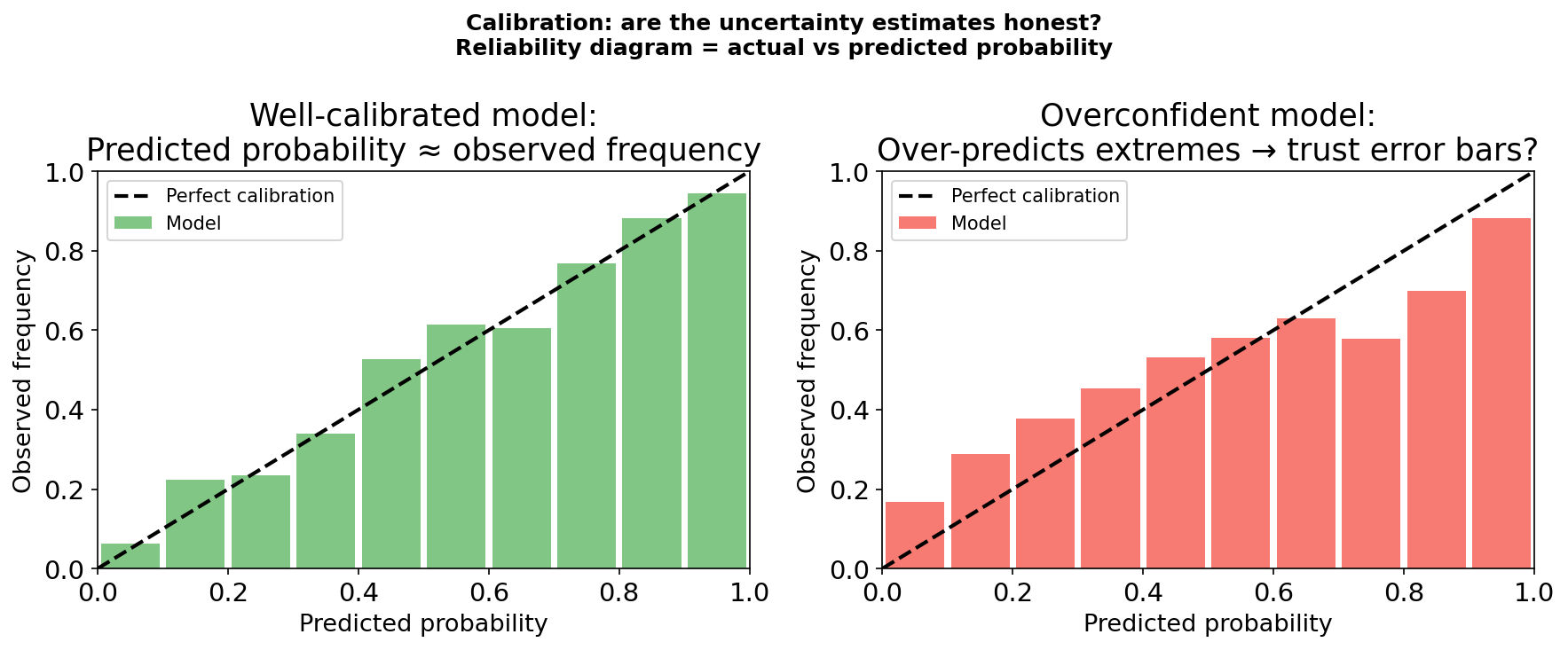
Calibration: are the error bars honest?

Left: a well-calibrated model — the predicted probability matches the observed frequency in each bin. Points scatter around the diagonal. Right: an overconfident model — predicted extremes (>90%, <10%) map to more moderate observed frequencies. This model’s error bars are too narrow: it is more wrong than it admits. The reliability diagram is the standard diagnostic.

• Walk through both panels. Left: every bar is approximately as tall as the diagonal. A 70% predicted probability yields ~70% of outcomes being positive. This model can be trusted — its number is what it says it is.
• Right: bars near 0.9 fall well below the diagonal. The model predicts 90% confidence but achieves only ~75% coverage. This model’s confident predictions are wrong more often than it thinks. Decision-makers who trust the 90% number will be surprised.
• The check: “a GP’s 95% band is calibrated IF the kernel is correct. If you fit an RBF kernel to data that has kinks, the model is misspecified and the 95% band may not achieve 95% coverage. A reliability diagram tells you this immediately.”
• How to fix it: temperature scaling (soft divide the logits), Platt scaling (sigmoid recalibration), or conformal prediction (guaranteed coverage regardless).

Calibration metrics and how to improve them

• Expected Calibration Error (ECE): average over bins of \(|(\text{predicted probability}) - (\text{observed frequency})|\). ECE = 0 is perfect. ECE > 0.1 is concerning.
• Reliability diagram: plot predicted probability vs observed frequency. A calibrated model follows the diagonal \(y=x\). Points above the diagonal = underconfident. Points below = overconfident.
• Temperature scaling: divide logits by learned scalar \(T > 1\) to soften predictions (\(T > 1\) reduces overconfidence). Applied post-hoc to a trained model — does not change the model.
• Conformal prediction as calibration: conformal wraps any model and guarantees coverage. It is the most principled post-hoc calibration: the calibration set is used to set the interval width exactly right.

• ECE is the standard metric in calibration papers. A well-calibrated model has ECE < 0.05. Most NN models without post-hoc calibration have ECE 0.10–0.30.
• Temperature scaling is the simplest fix: one scalar T, fit on the calibration set. It is the first thing to try. It fixes over/underconfidence globally but not per-input (it gives constant-width bands, like split conformal).
• Conformal is the strongest guarantee. Students who remember only one calibration tool should remember conformal: “split conformal wraps any predictor with a distribution-free coverage guarantee.”
• EM application: a segmentation network trained on 200 TEM images has ECE 0.18 — its 90% confidence predictions are wrong 28% of the time. Temperature scaling with T=1.3 reduces ECE to 0.04. Now the model is deployable.

Calibration: EM-specific considerations

• Domain shift destroys calibration. A GP or NN calibrated on Fe–O systems from one microscope may be badly calibrated on a different microscope (different aberrations, different detector gain, different specimen preparation). Always re-calibrate on data from the target instrument.
• The calibration set must match the test distribution. For EM: the calibration set should use the same microscope, sample preparation protocol, and acquisition settings as the intended deployment. A “calibration set” from a different lab is not a valid calibration set.
• Small calibration sets give wider (more conservative) intervals. Split conformal always guarantees coverage ≥ 1-α regardless of \(n_\text{cal}\). With small \(n_\text{cal}\) the intervals are slightly wider than necessary (conservative); with \(n_\text{cal} = 200\) the excess width is negligible. Use the largest feasible calibration set to get tighter, less wasteful intervals.
• Calibrate on outcomes, not residuals. For regression, check the reliability diagram using actual coverage fractions across the input domain, not just mean residuals.

• The domain shift point is the most practically important. Materials EM labs often train on one instrument and want to deploy on another. Without re-calibration, the uncertainty estimate is from the source instrument’s distribution — it says nothing about the target.
• The calibration-set matching requirement is a Weeks 4/7 callback: the GroupKFold / specimen-based split principle. The calibration set is, in effect, a held-out test set used for calibration. All the leakage rules from Week 4 apply: no specimen in both training and calibration.
• Small n_cal: split conformal guarantees marginal coverage ≥ 1-α (= 0.90) for ANY n_cal, given exchangeability. The (1+1/n_cal) factor inflates the quantile level so the discrete empirical quantile overshoots rather than undershoots — small n_cal means a slightly wider (more conservative) band, never undercoverage. With n_cal=50 the band is about 2% wider than the asymptotic width; with n_cal=200 the excess is ≈0.5%. Prefer larger calibration sets to get tighter (less wasteful) intervals, not to fix a coverage deficit that does not exist.

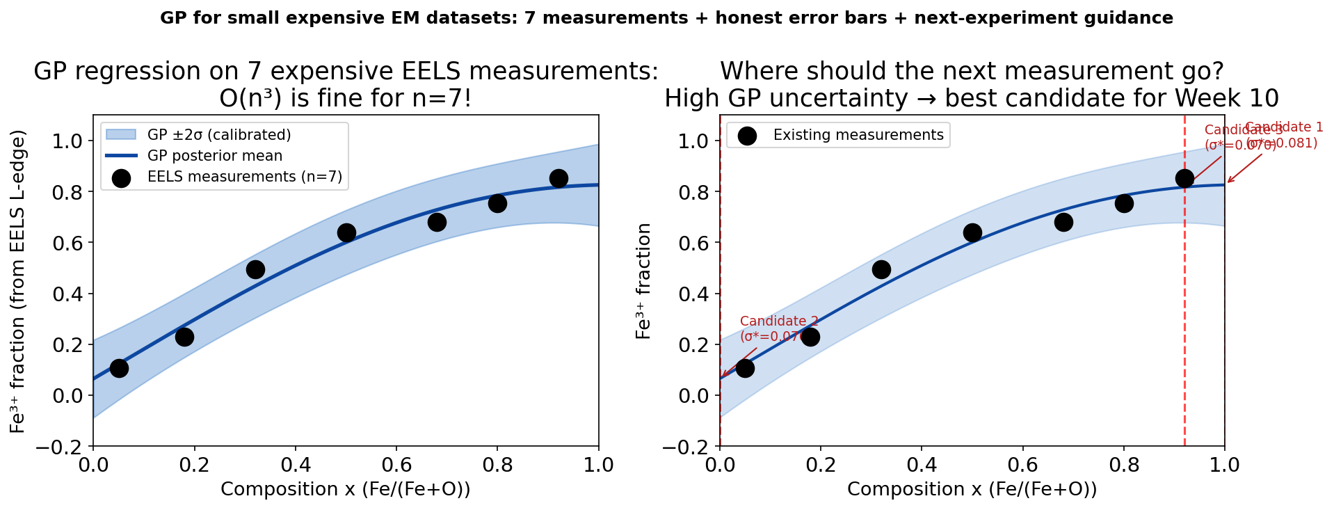
GP for small expensive EM datasets

Left: GP regression on 7 EELS measurements of Fe³⁺ fraction vs composition. The O(n³) cost is trivial for n=7. The posterior mean (blue) follows the S-curve; the ±2σ band (light blue) is tight in the measured region and wide beyond. Right: the three highest-uncertainty composition candidates for the next measurement are marked (red dashed lines). The GP tells the experimentalist where to measure next to reduce uncertainty most efficiently.

• This is the Week 9 / Week 10 bridge slide. Walk through both panels.
• Left: 7 EELS measurements, 1 hour per point = 7 hours of instrument time. The GP fits in milliseconds and gives calibrated error bars at all compositions — including those that were never measured. For a materials scientist, this is enormous value: one experiment session yields a predictive model for the entire composition space.
• Right: the active-learning candidates. The GP’s σ*(x) tells us the three compositions where uncertainty is highest. Measuring there will reduce the global uncertainty most efficiently. This is Week 10’s Bayesian optimisation / active learning framework.
• Practical notes: kernel selection for real EM data (Matérn-5/2 often better than RBF); normalise x to [0,1] and y to zero mean, unit variance before fitting; check calibration with a reliability diagram.
• Transition to forward link.

GP limitations and practical tips for EM

• \(O(N^3)\) cost: for \(N \leq 500\) EM measurements this is fast (< 1 s). For \(N \geq 2000\), use sparse GP approximations (inducing points) — available in GPyTorch and GPflow.
• Kernel choice matters: RBF assumes infinitely smooth functions. Materials property curves often have kinks (phase transitions). Try Matérn-5/2 (allows moderate roughness). Compare marginal likelihoods.
• Normalise inputs and outputs: GP kernels are scale-sensitive. Always centre and scale both \(x\) (to [0,1]) and \(y\) (to zero mean, unit variance) before fitting. De-normalise predictions afterwards.
• Multi-dimensional inputs (e.g. temperature × composition): the RBF kernel generalises to \(k(\mathbf{x},\mathbf{x}') = \sigma_f^2 \exp(-\frac{1}{2}(\mathbf{x}-\mathbf{x}')^\top \mathbf{L}^{-2}(\mathbf{x}-\mathbf{x}'))\) with a separate length-scale per dimension. This is Automatic Relevance Determination (ARD) — it down-weights irrelevant input dimensions.

• The sparse GP note: GPyTorch and GPflow both implement inducing-point sparse GPs that scale to N~10⁶. The idea is to summarise the N training points with M << N “inducing points” and compute the posterior approximately. Cost drops from O(N³) to O(NM²). For this course, M<=50 inducing points covers typical EM datasets.
• Matérn-5/2 practical note: sklearn’s kernel library includes Matern(nu=2.5). For materials property data, use it as the default instead of RBF. The extra smoothness parameter can be crucial for capturing abrupt property changes at phase boundaries.
• ARD is the GP’s way of doing feature selection: the optimised length-scale in each dimension reflects how important that dimension is. A large length-scale in dimension \(d\) means changing \(x_d\) has little effect on \(f\) — the data drove it to “not correlated.” This is dimensionality reduction as a by-product of GP fitting.

Forward link: Week 10 — Active & automated electron microscopy

• Today’s remaining gap: we have honest uncertainty estimates — the GP’s σ(x). Now we need a principled strategy for using* those estimates to guide acquisition.
• Week 10’s framework: Bayesian optimisation (BO) formalises the “measure where uncertainty is largest” intuition as an acquisition function — typically Upper Confidence Bound (UCB) or Expected Improvement (EI).
• BO loop for EM: (1) fit GP to current measurements; (2) optimise acquisition function to find next composition/condition; (3) measure; (4) update GP; (5) repeat until budget exhausted or convergence.
• The connection: today’s GP posterior is the model inside the BO loop. The GP uncertainty (σ) is the exploration signal. Week 10 adds the exploitation signal* (prefer high predicted values) and combines them into the acquisition function.
• Concrete EM payoff: with 20 budget measurements and a BO strategy, find the composition that maximises a target property (e.g. Fe³⁺ fraction ≥ 0.8) with fewer experiments than a grid search.

• Close the forward link explicitly: “today we learned to be honest about what we don’t know. Next week we learn to be efficient about filling in what we don’t know.”
• The BO loop is the algorithm that Week 10 will implement. Sketch it on the board: GP → acquisition function → new measurement → update GP. This loop runs autonomously on an automated EM instrument.
• UCB acquisition function: \(UCB(x) = \mu^*(x) + \kappa\sigma^*(x)\). The parameter \(\kappa\) controls exploration vs exploitation. \(\kappa=0\) is pure exploitation (always measure where the mean is highest). \(\kappa\to\infty\) is pure exploration (always measure where σ* is highest). Week 10 derives the right \(\kappa\).
• Close: “Today: uncertainty. Week 10: optimised uncertainty-guided acquisition. The GP posterior is the bridge.”

Notebook summary: Week 9 key results

• Dataset: 8 synthetic EELS measurements of Fe³⁺ fraction vs composition, Gaussian noise σ=0.03, random seed 42.
• Model: GaussianProcessRegressor (sklearn), RBF + WhiteKernel, optimised via log marginal likelihood (n_restarts_optimizer=10). Optimised kernel: \(0.476^2 \cdot \mathrm{RBF}(\ell=0.373) + \mathrm{WhiteKernel}(\sigma_n^2=0.000172)\).
• Uncertainty far vs near (SEED=42): predictive std at \(x_\mathrm{near}=0.659\) (dense training cluster) \(= 0.0145\); at \(x_\mathrm{far}=1.15\) (no data) \(= 0.1966\). Ratio: 13.5× — the band at the unexplored location is 13× wider.
• Adding a point at \(x=1.0\): reduces σ* at \(x_\mathrm{far}=1.15\) from 0.1966 to 0.1003 (49% reduction). Effect on x_near: +6.5% (negligible — far-away data barely affects nearby regions).
• Exercise: with fixed length-scale ℓ=1.2 (too long), the GP extrapolates with falsely narrow bands — the dangerous case. With ℓ=0.05 (too short), σ* inflates in every gap between adjacent points.
• Assert checks: all four pass on SEED=42: (1) std_far > std_near; (2) adding a point reduces std_far; (3) far-point has minimal effect near data; (4) far/near ratio > 5.

• All numbers on this slide must match the executed notebook exactly. If the notebook is re-run on different hardware with different sklearn version, update this slide before the next iteration.
• The 13.5× ratio is the key number students should remember: in the unexplored region, the uncertainty is an order of magnitude larger than at the data. That is what “uncertainty balloons” looks like numerically.
• The 49% reduction from adding one point is the active-learning payoff in numbers: one EELS measurement, 1 hour of instrument time, halves the uncertainty in the unexplored composition region. This is the quantitative argument for uncertainty-guided acquisition.
• Transition: “References.”

Continue

• → Next: Week 10 — Active & automated electron microscopy
• ← Back: Week 08 — Unsupervised learning & autoencoders for EM
• All courses

References

Pattern recognition and machine learning, Christopher M. Bishop.

Machine learning: A probabilistic perspective, Kevin P. Murphy.

Gaussian processes for machine learning, Christopher K. I. Williams & Carl Edward Rasmussen.

A gentle introduction to conformal prediction and distribution-free uncertainty quantification, Foundations and Trends in Machine Learning, Anastasios N. Angelopoulos & Stephen Bates.

Dropout as a Bayesian approximation: Representing model uncertainty in deep learning, Proceedings of the 33rd international conference on machine learning (ICML), Yarin Gal & Zoubin Ghahramani.

Simple and scalable predictive uncertainty estimation using deep ensembles, Advances in neural information processing systems, Balaji Lakshminarayanan, Alexander Pritzel, & Charles Blundell.