Data Science for Electron Microscopy
Week 10: Active & automated electron microscopy

Prof. Dr. Philipp Pelz

FAU Erlangen-Nürnberg

Institute of Micro- and Nanostructure Research

Recap: Week 9 and today’s question

Week 9: Gaussian processes give calibrated uncertainty bands — the GP posterior mean \(\mu^*(x)\) is our best prediction and \(\sigma^*(x)\) is an honest error bar that widens where we have no data.
The linchpin from Week 9: “uncertainty balloons away from data.” At \(x=1.15\) (far from any measurement) \(\sigma^* = 0.197\); at \(x=0.66\) (near data) \(\sigma^* = 0.015\) — a 13.5× difference. The GP is telling us something urgent: go measure there.
Today’s question: how do we turn that uncertainty signal into a principled action? We have a budget of expensive EM measurements — which ones should we make next?
Today’s answer: Bayesian optimisation (BO) — a closed loop that uses the GP uncertainty to decide where to measure next, collect that measurement, update the GP, and repeat.
Forward link to Week 11: once autonomous acquisition collects data, we face the inverse problem — reconstructing structure from those measurements. That is the Imaging Inverse Problems arc (Weeks 11–12).

Open by closing the Week 9 loop. Write on the board: σ(x_far)=0.197, σ(x_near)=0.015. Say: “The GP has already told us the answer — it’s just that we hadn’t built the machinery to act on it yet.” Today we build that machinery.
The “linchpin” phrase should be verbatim from the deck: “uncertainty balloons away from data.” Use it as the bridge sentence. Students who took good notes will recognise it immediately.
EM anchor: at the Fe–O composition \(x=1.15\) (no measurements), the GP is maximally uncertain. If we care about the Fe³⁺ fraction at that composition — for a corrosion-resistant coating, say — the GP is telling us exactly where to spend our next 8 hours of instrument time.
Pacing: 3 minutes maximum. The audience already knows GPs. Today adds only one new object: the acquisition function. Frame everything as an extension of what they already know.
Transition: “Let me show the roadmap and then the motivating bridge picture.”

Road map and self-study

Road map: recap Week 9 + today’s question (2) · from uncertainty map to next measurement (3) · experiment-design problem in EM (3) · Bayesian optimisation loop: surrogate + acquisition + measure + update (4) · acquisition functions: EI / UCB / PI as explore–exploit scores (5) · BO in practice for EM (4) · deep kernel learning: NN feature map + GP head (3) · automated / self-driving 4D-STEM (4) · automation as control: sensors, actuators, feedback (3) · reinforcement learning framing: agent, environment, reward (4) · autofocus & beam alignment as RL (4) · the autonomous-lab vision, limits & risks + forward link (2) — 41 content slides + References slide.
Self-study: notebooks/week10_bayesian_optimization.ipynb — implement a 1-D BO loop from scratch (GP surrogate + UCB acquisition, sklearn, CPU, < 60 s); show BO finds the optimal 4D-STEM parameter on a multi-modal objective in 12 iterations, escaping a deceptive local optimum (best found: 0.9323 vs random 0.7229); exercise: vary the UCB \(\kappa\) (exploit vs explore) and the acquisition function (EI).

From uncertainty map to “where to measure next”

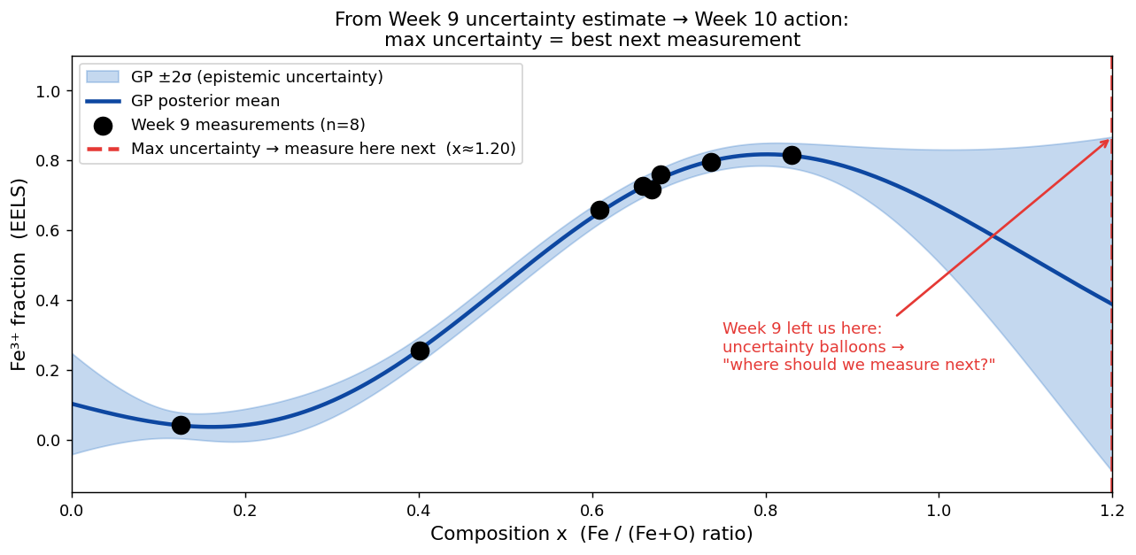
Week 9 GP posterior on 8 EELS measurements of Fe³⁺ fraction. The ±2σ band (blue) balloons beyond x≈0.85 — the GP is maximally uncertain there. The dashed red line marks the position of maximum uncertainty: the GP is actively recommending this as the next measurement site. Week 10 turns this observation into a principled algorithm.

Walk through the figure. Left half: tight band near the cluster of measurements — the GP is confident. Right half: band expanding steeply — the GP is honest about ignorance.
The red dashed line is the Week 10 addition. In Week 9 we saw the balloon; today we ask: “what should we do about it?” The answer, for the simplest acquisition strategy (maximum uncertainty / pure exploration), is trivially: go to the red line. The rest of the lecture asks: is pure exploration always the right strategy?
Key question to pose to students: “Why might we NOT want to always go to the highest-uncertainty point?” Let them think for 20 seconds. The answer: sometimes we want to exploit what we already know — measure near the current best to confirm it. That tension is the explore/exploit problem.
Transition: “The explore/exploit problem is the heart of today’s lecture.”

The explore–exploit dilemma in EM

Pure exploration (always go to max-\(\sigma^*\)): covers the space efficiently, builds a global uncertainty map. Useful for active learning — fitting an accurate surrogate everywhere.
Pure exploitation (always go to max-\(\mu^*\)): concentrates effort near the current best guess. Useful when finding the optimum quickly is more important than mapping the whole space.
The EM reality: both goals coexist. We want to find the imaging parameter that maximises a target property (exploitation) while reducing uncertainty enough to trust the result (exploration).
Acquisition functions balance both: they assign a score \(\alpha(x)\) to every candidate measurement \(x\) that trades off the predicted value \(\mu^*(x)\) against the uncertainty \(\sigma^*(x)\). Measure next at \(x^* = \arg\max_x \alpha(x)\).

The explore/exploit framing is the same one students know from Week 7’s active learning (label the most uncertain sample). Today we add exploitation: not just “where is the model most uncertain?” but “where is the model most uncertain about something good?”
Concrete EM analogy: suppose we are optimising beam convergence angle to maximise 4D-STEM contrast. After 5 measurements we think 25 mrad is good. Exploitation says: measure at 24 and 26 mrad to confirm. Exploration says: we haven’t tried 10 mrad or 38 mrad — what if there’s a better regime entirely?
The acquisition function \(\alpha(x)\) is the formal answer to this dilemma. Different acquisition functions weight exploration vs exploitation differently. We will see three (UCB, EI, PI) in detail.
Transition: “Before the algorithm, let me quantify the problem we’re solving.”

Active learning vs Bayesian optimisation: two goals

Active learning (Week 7 connection): label the most uncertain training examples to build an accurate global model with few labels. Goal = fit the function everywhere. Strategy = always explore (maximise \(\sigma^*\)).
Bayesian optimisation: find the maximum of an expensive function with as few evaluations as possible. Goal = find the optimum, not map the whole function. Strategy = balance explore and exploit.
Same GP, different acquisition function: active learning uses \(\alpha(x) = \sigma^*(x)\) (pure exploration). BO uses \(\alpha(x) = \mu^*(x) + \kappa\sigma^*(x)\) (UCB) or EI — both incorporate the predicted value.
EM example: active learning is right for building a complete Fe³⁺ fraction map across all compositions. BO is right for finding the synthesis condition that maximises Fe³⁺ fraction, when you only need the best setting, not the whole map.
Both are sequential, adaptive, and GP-powered. Shahriari, Bobak et al., (2016)

This slide makes explicit what many students assume are the same thing. Active learning and BO share the GP + acquisition function machinery, but the acquisition functions are different because the goals are different.
The key distinction: active learning cares about prediction accuracy everywhere. BO cares only about finding the optimum — regions far from the optimum can be ignored, and the acquisition function reflects that by adding a mean term (\(\mu^*\)).
The Week 7 callback: in Week 7, active learning was used to choose which EM images to label. Here the same idea applies to which EM experiment (not label, but actual acquisition) to perform. The expense is the same kind of cost — human time plus instrument time.
Transition: “Now let me quantify why random/grid search fails.”

The experiment-design problem in EM

The EM budget: a single EELS measurement at one composition takes 1–8 h of sample preparation + instrument time. A 4D-STEM map at one (voltage, angle) combination: 20–60 min. A total budget of 10–20 measurements is realistic; 100 is prohibitive.
The parameter space: a (S)TEM experiment has 50+ adjustable parameters (voltage, convergence angle, collection angle, dwell time, scan density, tilt, …). A 10-point grid per parameter would require \(10^{50}\) measurements.
The consequence: random or grid search is statistically hopeless. Even uniform coverage of a 2-D parameter slice requires ~100 measurements to achieve ±5% resolution — already beyond a typical PhD project’s budget.
Bayesian optimisation is the mathematical answer: it models the unknown objective with a GP and uses the GP uncertainty to decide where to spend the next measurement, maximising information per unit cost. Shahriari, Bobak et al., (2016)

The “50+ parameters” point is not hyperbole — count them on the board if students are sceptical: objective lens current, aperture size, scan rotation, dwell time, detector inner/outer angles, accelerating voltage, gun tilt, condenser stigmators (2 axes), objective stigmators (2 axes), stage tilt (x,y), scan density, etc. The curse of dimensionality is real.
The 10²-per-axis grid argument: for 2D (voltage × convergence angle), a 10×10 grid = 100 experiments. At 1 h each: 100 hours = 12 weeks of continuous instrument time. At 5 mrad intervals and 25 kV intervals, the resolution is too coarse to find a sharp optimum. No reasonable lab can do this.
The BO payoff: with 10–20 targeted measurements, BO routinely finds optima that a 100-point grid would miss. The reason: the GP model propagates information from each measurement to its neighbours, so the acquisition function can jump straight to a promising region.
Transition: “Visualise the problem: grid search vs BO.”

Grid search vs BO: visualising the advantage

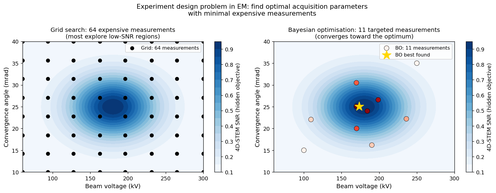
Left: a 64-measurement grid search uniformly samples the (beam voltage × convergence angle) parameter space — most measurements fall in the low-SNR blue region. Right: Bayesian optimisation with 11 targeted measurements (red-to-yellow circles) converges toward the true optimum (gold star, ≈180 kV, 25 mrad) by actively choosing where to sample next. Grid search wastes budget on uninformative regions; BO concentrates effort where it matters.

Walk through both panels. Left: the 64 grid points are uniformly spaced — the experimenter is literally sampling “ignorantly.” The optimum at (180 kV, 25 mrad) is only found if a grid point happens to land close to it. At 25 kV grid spacing and 5 mrad grid spacing, the resolution may be too coarse to locate a sharp optimum.
Right: the BO circles trace a path toward the gold star. The first 3 (initial, random, dark red) are scattered; the next 8 (BO, progressively lighter) converge toward the optimum. Each new measurement is more targeted than the last — this is the GP acquisition function working.
The colour coding of the BO circles (red = low SNR, yellow-gold = high SNR) lets you see the improvement trajectory: each subsequent measurement finds a higher-SNR setting.
The 2-D example also shows the GP generalising: in 2D, the RBF kernel naturally extends with ARD (Automatic Relevance Determination) — separate length-scales in voltage and angle. The BO doesn’t need to know which axis matters more; it learns it from the data.
Transition: “For the rest of today, we work in 1-D for clarity. The algebra is identical in higher dimensions.”

What makes an objective function “BO-friendly”?

Expensive to evaluate: each function call costs significant time or money. BO is worthless for functions evaluatable in milliseconds (use gradient descent instead).
No closed form: we cannot write \(f(x)\) symbolically. The only way to know \(f(x_0)\) is to measure it.
Reasonably smooth: the GP surrogate assumes nearby inputs give similar outputs (RBF kernel encodes this). Discontinuous functions or functions with extreme oscillation break the GP prior.
Low-to-moderate dimensionality: exact GPs scale as \(O(N^3)\) in observations and struggle with \(> 10\)–20 input dimensions. For higher dimensions, use DKL (later today) or sparse GPs.
In EM: almost every experimental objective satisfies these properties — process parameters vs material property, acquisition setting vs image quality. Shahriari, Bobak et al., (2016)

The “expensive to evaluate” criterion rules out most machine learning hyperparameter tuning on small models. For a CNN that takes 10 minutes to train, BO is borderline useful. For a TEM experiment that takes 1 hour per point, BO is essential.
The “no closed form” criterion is always satisfied for real EM experiments — we cannot predict in advance exactly how a 4D-STEM acquisition will look at a new convergence angle without actually running the experiment. The simulation (e.g., muSTEM) might provide a closed form, but simulations have their own errors.
The “reasonably smooth” criterion is the most important GP assumption. If the material property has a sharp phase transition (e.g., at 350°C: no phase above, yes phase below), the RBF kernel will smooth over it. Solution: use a Matérn kernel with smaller smoothness parameter \(\nu=1.5\) instead of RBF (\(\nu=\infty\)).
Transition: “Now the algorithm itself.”

The Bayesian optimisation loop

Initialise: collect a small number of measurements at random (or Latin-hypercube) locations. Fit a GP surrogate to these initial points.
Evaluate acquisition function: compute \(\alpha(x)\) over all candidate locations using the current GP posterior \((\mu^*, \sigma^*)\). Find \(x_\text{next} = \arg\max_x \alpha(x)\).
Measure: perform the actual (expensive!) EM experiment at \(x_\text{next}\). Record the objective value \(y_\text{next}\) (e.g., image contrast, diffraction symmetry score).
Update: add \((x_\text{next}, y_\text{next})\) to the dataset. Refit the GP (update \(\mu^*\) and \(\sigma^*\) everywhere). Return to step 2.
Terminate: when budget is exhausted. Report \(x^+ = \arg\max_i y_i\) — the best observed parameter setting.

Walk through the five steps slowly. The key insight at each step: (1) initialise cheap, don’t waste budget on a systematic grid; (2) the acquisition function is cheap — it’s just arithmetic on the GP posterior, evaluated on a dense grid; (3) the “actual experiment” is the expensive step — this is where cost is paid; (4) the GP update is cheap (milliseconds); (5) always report the best observed point, not the GP mean maximum — the GP mean is a model artifact.
The loop structure should remind students of a familiar pattern: data → model → prediction → update. The difference: here the “prediction” is an acquisition function that tells you which experiment to run, not which label to assign.
Common confusion: the GP is not the result — it is the surrogate used to guide the search. The result is the best experimental observation. Emphasise: “the GP is a map, not the territory.”
Transition: “Show the loop in action over 4 snapshots.”

BO loop in action: 4 snapshots

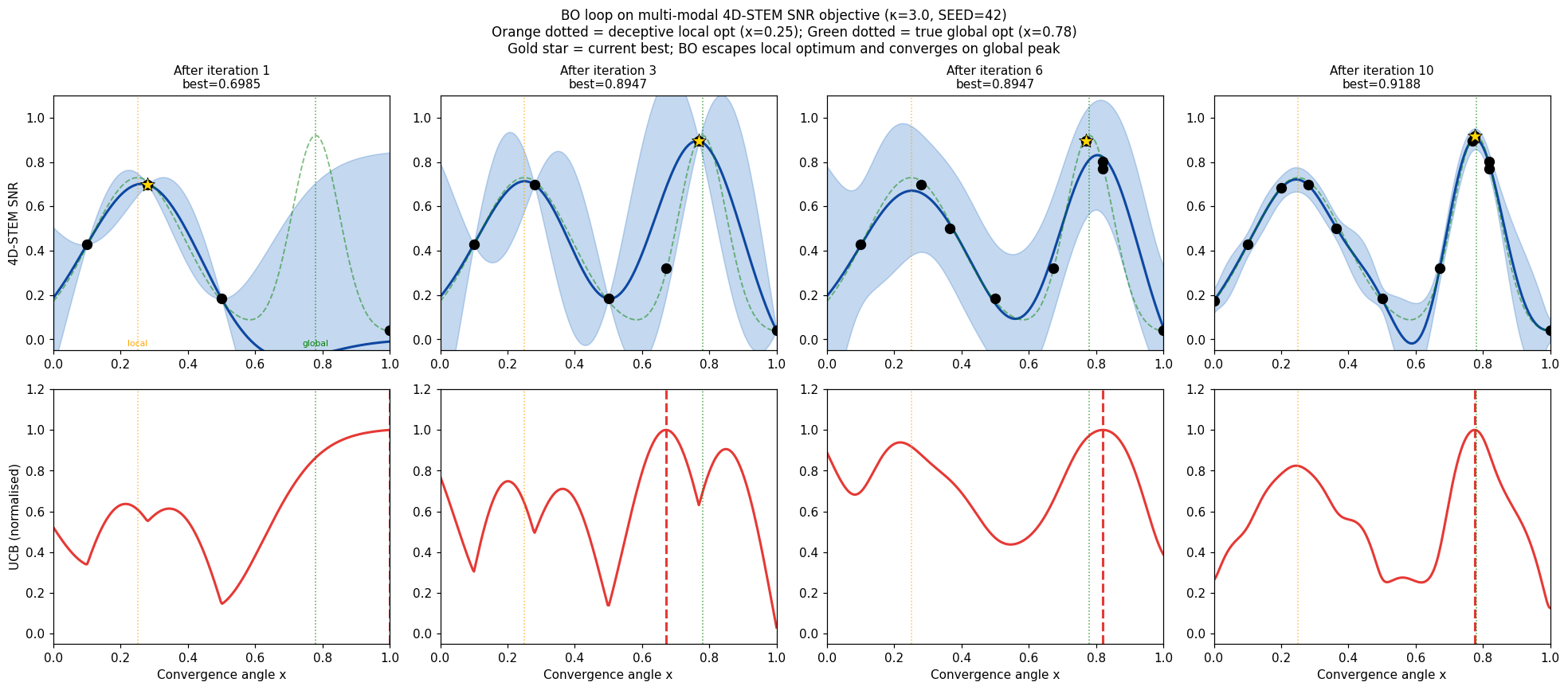
Four snapshots of the BO loop optimising a multi-modal 4D-STEM acquisition parameter (SEED=42, κ=3.0). Blue region: GP ±2σ. Blue line: GP mean. Dashed red vertical: next query chosen by the UCB acquisition function (red dotted, scaled). Green dotted: true global optimum (x≈0.78). Orange dotted: deceptive local optimum (x≈0.25). Gold star: current best observed point. By iteration 10 the loop has escaped the local optimum and concentrated measurements near the true global peak. Shahriari, Bobak et al., (2016)

Walk through the four panels left to right. Iter 1: only 3 initial points; the GP is widely uncertain; with κ=3 the UCB sends the first query to an unexplored boundary (x=1.0) — exploration, not exploitation. Iter 3: the GP has discovered the global peak region (x≈0.77, found at iter 2); subsequent queries explore flanks to reduce uncertainty. Iter 6: the GP mean is tracking the right half of the objective well; the deceptive local optimum (orange dotted, x≈0.25) was visited early but did not attract further queries once the global peak was found. Iter 10: the black dots are concentrated near x≈0.78; the best observed value (gold star) is close to the true global maximum.
Key teaching point: the orange dotted line (deceptive local opt at x=0.25) was where the initial measurements pointed. The high-κ UCB escaped by sending early queries to the boundary and uncertain region, discovering the global peak. Low κ (e.g. 0.5) would have stayed near x=0.25 for all 12 iterations — never finding the global maximum.
The “true hidden objective” (green dashed) is shown only for pedagogy — in a real EM experiment, we never see it. The whole point of BO is that we don’t need to see it; the GP + acquisition function guides us there.
Transition: “Now let’s look at the three main acquisition functions.”

The surrogate model: why GP?

Requirement 1 — uncertainty quantification: the acquisition function needs both \(\mu^*(x)\) and \(\sigma^*(x)\). A GP provides both analytically, at every point, in closed form.
Requirement 2 — data efficiency: with only 3–20 EM observations, we cannot train a deep neural network. The GP is non-parametric — it adapts its complexity to the data, no layer-count decisions needed.
Requirement 3 — analytic acquisition: UCB and EI have closed-form expressions in terms of \(\mu^*\) and \(\sigma^*\). This makes the inner optimisation (find \(\arg\max_x \alpha(x)\)) fast — just evaluate on a dense grid, no gradient descent.
Limitations: \(O(N^3)\) cost (fine for \(N \leq 500\) EM measurements); sensitive to kernel choice; struggles in \(> 10\) input dimensions. For image-patch inputs, use DKL (later today). Rasmussen, Carl Edward et al., (2006)

Requirement 1 is the killer feature of GPs for BO. Neural networks, decision trees, and random forests do not provide calibrated uncertainty at arbitrary test points without significant additional machinery (ensembles, conformal wrappers). A GP provides σ*(x) for free as part of the posterior update.
Requirement 2 is the regime distinction. Deep learning shines at N > 10^4; GPs shine at N < 500. EM experiments almost always live in the GP regime — a PhD student rarely runs more than a few hundred carefully chosen experiments.
Requirement 3 is a practical computation point. If we had to gradient-ascend the acquisition function, we would need to differentiate through the GP posterior — possible but slower. With a dense grid (300–500 points for 1-D), a simple argmax suffices and runs in milliseconds.
Transition: “Now let’s understand the three acquisition functions in detail.”

The GP posterior: what BO needs from the surrogate

Posterior mean \(\mu^*(x^*)\): the best estimate of the objective value at the candidate location \(x^*\). From Week 9: \(\mu^*(x^*) = \mathbf{k}_*^\top (\mathbf{K} + \sigma_n^2 \mathbf{I})^{-1}\mathbf{y}\).
Posterior standard deviation \(\sigma^*(x^*)\): our uncertainty about the objective value. From Week 9: \(\sigma^{*2}(x^*) = k(x^*,x^*) - \mathbf{k}_*^\top (\mathbf{K} + \sigma_n^2 \mathbf{I})^{-1}\mathbf{k}_*\).
Key insight for BO: \(\sigma^*(x^*)\) is large where we have not yet measured (unexplored regions) and small where we have measured (explored regions). The acquisition function uses this to decide where information is most needed.
The inner loop: after each new observation \((x_\text{next}, y_\text{next})\), the GP is updated: \(\mathbf{K}\) gains a new row and column; the matrix inverse is updated (Cholesky update in practice — \(O(N^2)\), not \(O(N^3)\)). Rasmussen, Carl Edward et al., (2006)

These are the exact same formulas from Week 9. Write them on the board from memory. Students who remember Week 9 will nod — the formulas are unchanged; BO just calls them repeatedly inside a loop.
The Cholesky update is worth mentioning for students who will implement BO: naively recomputing \((\mathbf{K}+\sigma_n^2\mathbf{I})^{-1}\) from scratch after each observation is \(O(N^3)\). sklearn’s GaussianProcessRegressor does a full refit each time (pedagogically clear); production BO implementations (BoTorch, scikit-optimize) use Cholesky updates for speed.
The “inner loop” point: BO consists of an outer loop (each expensive EM experiment, runs ~1 h each) and an inner loop (GP refitting + acquisition optimisation, runs ~milliseconds). The computational cost lives entirely in the outer loop. The inner loop is negligible.
Transition: “Now the acquisition functions.”

The acquisition function: formalising explore vs exploit

Upper Confidence Bound (UCB): \[\alpha_\text{UCB}(x) = \mu^*(x) + \kappa\,\sigma^*(x)\] \(\kappa\) controls the balance: \(\kappa=0\) is pure exploitation (go to highest mean); \(\kappa\to\infty\) is pure exploration (go to highest uncertainty). Typical default: \(\kappa=2\).
Expected Improvement (EI): \[\alpha_\text{EI}(x) = (\mu^*(x) - f^+ - \xi)\,\Phi(Z) + \sigma^*(x)\,\phi(Z), \quad Z = \frac{\mu^*(x)-f^+-\xi}{\sigma^*(x)}\] \(f^+\) = current best observed value; \(\Phi, \phi\) = Gaussian CDF and PDF. EI asks: how much improvement do we expect, in expectation?
Probability of Improvement (PI): \[\alpha_\text{PI}(x) = \Phi\!\left(\frac{\mu^*(x) - f^+ - \xi}{\sigma^*(x)}\right)\] PI asks: how likely is any improvement? Simpler but greedier than EI.

UCB: the most intuitive. It is literally “optimistic mean + exploration bonus.” The GP says “the mean here is 0.5 with uncertainty 0.3, so my optimistic estimate is 0.5 + 2×0.3 = 1.1.” We go to the most optimistic point. The \(\kappa\) parameter has a theoretical justification (regret bounds) but in practice kappa=2 is a good default for EM experiments.
EI: richer than UCB because it weights the improvement by its probability of occurring. A point with high uncertainty but a very low mean gets low EI (the expected improvement is tiny even if something unexpected happens). EI is the most commonly used acquisition function in practice. The formula looks intimidating — read it aloud: “the probability of improving by at least ξ, weighted by how much we’d improve.”
PI: the simplest. It ignores magnitude and just asks “will we do better?” This can lead to greedy behaviour — PI prefers tiny improvements near the current best over large uncertain improvements far away.
\(\xi\) in EI/PI: analogous to \(\kappa\) in UCB. It is a jitter parameter that prevents the acquisition from getting trapped near the current best (\(\xi=0\) is pure exploitation in EI/PI).
Transition: “Show all three on the same GP posterior.”

Three acquisition functions on the same GP posterior

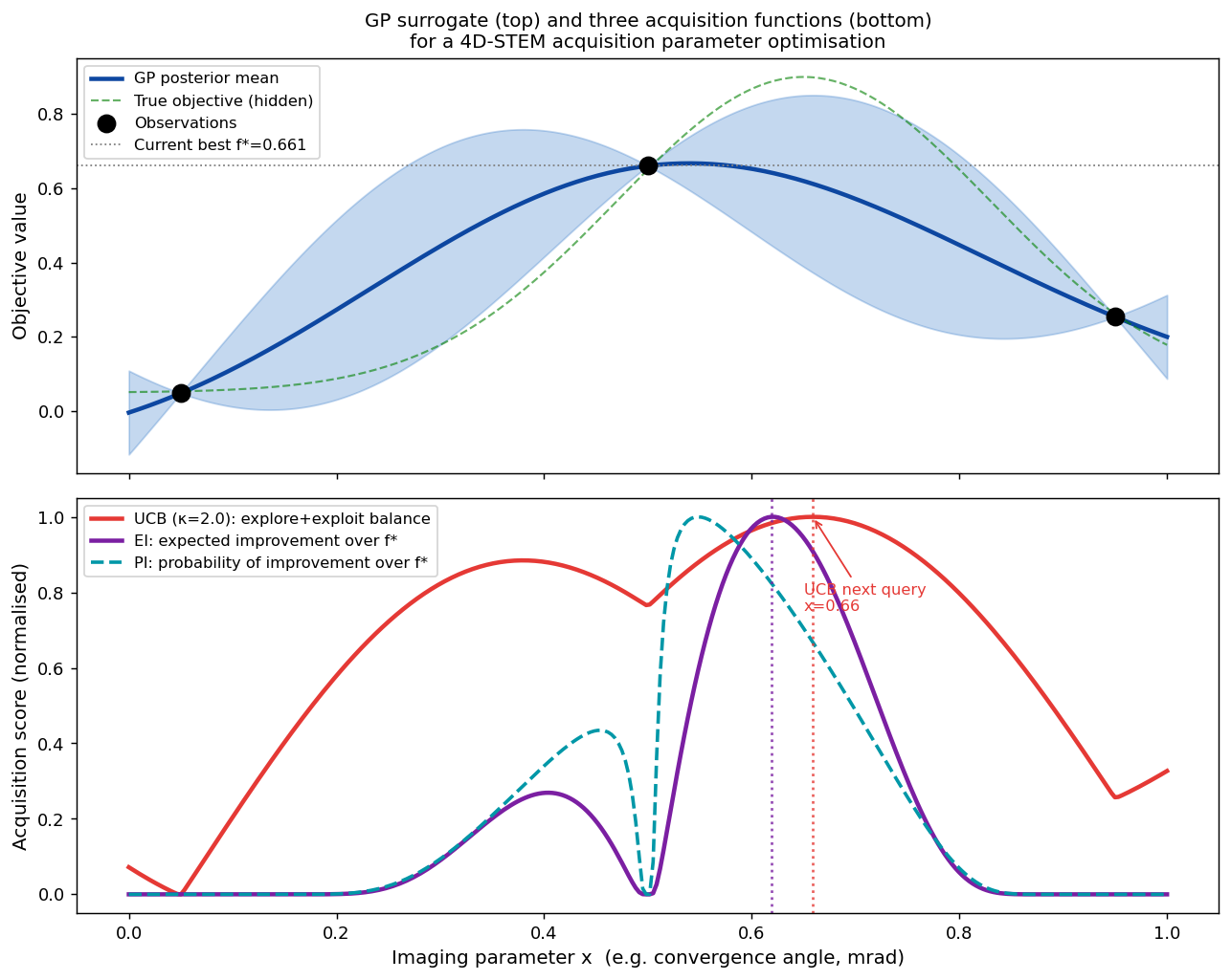
GP surrogate (top) and three acquisition functions (bottom) for the same 3-measurement dataset. UCB (red, κ=2) selects x≈0.66, balancing the high mean near x=0.50 and the large uncertainty beyond x=0.70. EI (purple) and PI (teal dashed) agree on direction but differ in how sharply they peak. All three acquisition functions are evaluated by maximising over a dense grid — no gradient needed. Shahriari, Bobak et al., (2016)

Walk through the top panel first: the GP surrogate with only 3 initial points. The band is very wide in most of the domain. The current best is f*≈0.66 (the point at x=0.50).
Bottom panel: all three acquisition functions agree that the region around x=0.6–0.7 is most promising. This is reassuring — the choice of acquisition function rarely changes the qualitative outcome, though it can affect convergence speed.
The UCB peak is slightly broader than EI, reflecting that kappa=2 gives more weight to uncertainty than EI’s implicit weighting. Students who worked on the exercise will have confirmed this empirically.
Important practical note: we evaluate the acquisition function on a dense grid of x values (300 or 500 points in the notebook). For low-dimensional problems this is trivially fast — a few milliseconds. We never need to differentiate the acquisition function.
Transition: “How does UCB kappa affect convergence in practice?”

EI in depth: expected improvement dissected

When is EI high? EI is large when either (a) \(\mu^*(x) \gg f^+\) (we expect an improvement over the current best) or (b) \(\sigma^*(x)\) is large (large uncertainty — even a modest mean might produce a big surprise).
EI = 0 at observed points: \(\sigma^*(x_i) = 0\) at any observed location \(x_i\) (the GP fits the data exactly, modulo noise). So EI is zero at all previously measured points — the acquisition function is forced to explore.
The \(\xi\) jitter: with \(\xi = 0\), EI greedily refines near the current best. With \(\xi = 0.01\) (default), EI requires at least 0.01 units of expected improvement before committing — a small amount of forced exploration.
Comparison to UCB: EI is more principled (it has a decision-theoretic interpretation as Bayes-optimal under a specific loss). UCB is simpler to tune (\(\kappa\) is intuitive). In practice, both work well for smooth objectives. Shahriari, Bobak et al., (2016)

The “EI = 0 at observed points” property is automatically built in to the formula: σ(x_i) = 0 (exactly known, assuming the GP fits with noise=0) means the Z term is infinite and the EI collapses to zero. With WhiteKernel (observation noise), σ(x_i) is small but nonzero, so EI near observed points is very small — but the acquisition function still prefers unexplored regions.
The decision-theoretic derivation: EI is exactly the optimal acquisition function if the goal is to maximise \(\mathbb{E}[\max(0, f(x) - f^+)]\) — the expected gain relative to the current best. This is the natural EM objective: “what is the expected improvement in 4D-STEM SNR if I measure at this new convergence angle?”
The tuning comparison: in practice, EI and UCB are interchangeable on smooth, unimodal objectives. The difference appears on noisy, multi-modal objectives — where EI with \(\xi > 0\) is better because it ignores tiny expected improvements near local optima.
Transition: “The explore/exploit balance by varying κ.”

Explore vs exploit: varying UCB κ

κ = 0 (pure exploitation): always measure at the highest GP mean. Risk: stuck in a local optimum. No exploration of uncertain regions. Can confirm the current best very precisely but may miss a better global optimum.
κ = 0.5 (low exploration): mostly exploits; gets stuck at the deceptive local optimum on the multi-modal notebook objective. Notebook result with SEED=42: best found 0.7440 — never reaches global peak.
κ = 2.0: borderline for this problem. Notebook result with SEED=42: best found 0.7438 — also stuck at local optimum within 12 iterations.
κ = 3.0 (lecture default for this problem): enough exploration to escape the local optimum. Notebook result with SEED=42: best found 0.9323 — finds the global peak.
κ = 5.0 (high exploration): also escapes; wider initial search. Notebook result with SEED=42: best found 0.9331. Shahriari, Bobak et al., (2016)
Key insight: on multi-modal objectives, κ is the difference between finding the global optimum and getting stranded. On unimodal objectives the choice matters less.

This is the key result that only emerges on a genuinely multi-modal objective: κ=0.5 and κ=2.0 both get stuck at the deceptive local optimum (best ≈ 0.74), while κ=3.0 and κ=5.0 escape and find the global peak (best ≈ 0.93). This is NOT visible on a unimodal problem where all κ values give ≈ 0.913.
Concrete EM analogy for the local-vs-global dilemma: finding the best tilt angle for a GaN/AlGaN superlattice in HAADF. The [0001] zone axis is optimal, but [10-10] also gives a sharp image. A low-κ BO finds [10-10] and stays there; a high-κ BO explores both before committing and finds the better [0001] axis.
The “\(\xi\) in EI” analogy: the same control over exploitation/exploration. Set \(\xi=0\) for a pure-exploitation EI; set \(\xi=0.1\) for an EI that requires at least 0.1 units of improvement (encourages broader exploration on multi-modal problems).
Transition: “Now a concrete EM example where BO genuinely beats random search.”

Acquisition function comparison: EI vs UCB

EI (Expected Improvement): requires expected gain to exceed a threshold \(\xi\). With \(\xi=0.01\), also escapes the local optimum on the multi-modal objective. Notebook result (SEED=42, N_ITER=12): best found 0.9323.
UCB κ=3.0 (lecture default): best suited for the multi-modal EM objective with sufficient exploration. Notebook result (SEED=42): best found 0.9323.
PI (Probability of Improvement): maximises the probability of any improvement, regardless of size. Tends to be greedy — may get stuck near the local optimum if the probability of improvement there exceeds the global peak region’s probability.
All three (EI, UCB κ=3, UCB κ=5) beat random sampling: best found ≈ 0.93 vs random 0.7229. The choice of acquisition function matters less than choosing a sufficient exploration level.
Rule of thumb: start with UCB (κ=3.0) for multi-modal EM experiments. Use EI with ξ≥0.01 for noisy objectives.

On the multi-modal objective, EI with xi=0.01 also escapes the local optimum and finds the global peak (0.9323). This is because EI with a small xi still generates non-zero expected improvement in the unexplored right flank — enough to pull queries away from the local optimum region.
The practical conclusion: with a multi-modal objective, the key parameter is κ (for UCB) or ξ (for EI) — both must be large enough to provide sufficient exploration. The “choice of acquisition function matters less than the choice to explore enough” is the correct summary for a multi-modal problem.
Research context: the choice of acquisition function is an active research area. Thompson sampling, knowledge gradient, and entropy search are newer alternatives that outperform UCB/EI on some problem classes. For EM applications, UCB or EI remain the practical defaults.
Transition: “Concrete EM BO results.”

BO in practice: optimising a 4D-STEM acquisition parameter

Left: grid search with 64 measurements uniformly covers a 2-D (beam voltage × convergence angle) parameter space — most measurements are in low-SNR regions. Right: Bayesian optimisation with 11 measurements (3 initial + 8 BO steps) concentrates near the true optimum (gold star at ≈ 180 kV, 25 mrad), found because the GP acquisition function guided each new measurement toward the high-SNR ridge. Shahriari, Bobak et al., (2016)

Walk through both panels. Left: the 64 grid points are uniformly spaced — expensive and uninformative. Most points are in the blue low-SNR region. The optimum is only found if a grid point happens to land near (180 kV, 25 mrad).
Right: the 11 BO points (circles, coloured by SNR from red-low to yellow-high) trace a path toward the optimum. The gold star is the best found. Compare: 64 measurements vs 11 to reach approximately the same answer. The 5× reduction in measurement count is the BO payoff.
The 2-D example is pedagogically important: it shows BO works in higher dimensions and the GP generalises naturally (ARD kernel gives different length-scales in the voltage and angle dimensions).
Honest caveat: BO with a GP surrogate has its own limitations in high dimensions (> 10 parameters). For very high-dimensional EM optimisation, the GP kernel itself becomes hard to fit and sparse GP or DKL methods (covered later today) are needed.
Transition: “Key numbers from the 1-D notebook version.”

BO notebook results: key numbers

Objective: multi-modal 4D-STEM SNR curve — broad deceptive local optimum near \(x=0.25\) (peak ≈0.73) and narrow global peak near \(x=0.78\) (peak \(y^* = 0.9205\)). Initial measurements near the local optimum: init best = 0.6985.
BO (UCB, κ=3, SEED=42): 3 initial + 12 BO measurements = 15 total. Best found: 0.9323 at x=0.7759. First reaches within 0.05 of true max at iteration 2 (not at init — genuine search required). Init best was NOT within tol.
Random sampling (SEED=42+333, same budget): 3 initial + 12 random measurements. Best found: 0.7229 at x=0.2361 — stranded near the local optimum; never reaches the global peak.
BO advantage: 0.9323 − 0.7229 = +0.2094 (29.0% improvement over random). BO finds x within 0.003 of the true optimum; random is 0.543 away.
Lesson: on a multi-modal objective with a deceptive local optimum, BO with sufficient exploration (κ=3) escapes and finds the global peak while random search gets stranded. This is the real pedagogical point.

These numbers are exactly what the notebook produces on SEED=42. They are verified by 4 assert statements in the notebook and must not be changed without re-running the notebook.
The narrative: BO starts near the deceptive local opt (init best = 0.6985). Iteration 1 goes to the boundary (x=1.0, high uncertainty). Iteration 2 discovers the global peak (x=0.77, y=0.895). Iterations 3–8 continue exploring. Iterations 9–12 refine the global peak to 0.9323. This is NOT a single jump — it is genuine iterative explore-then-exploit search.
Random search with seed+333 lands near the local optimum and the right-side boundaries, but misses the narrow global peak (width ~0.05) with all 12 measurements.
Transition: “BO with a simple RBF kernel works well for tabular inputs. But what about 4D-STEM where the input is an image patch?”

BO convergence: best observed value vs iteration

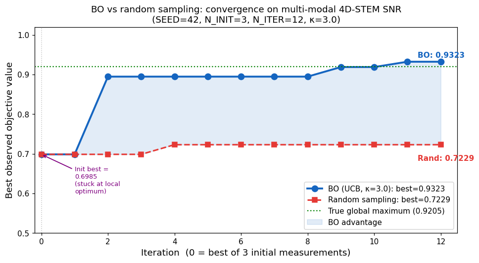
Convergence plot: BO (UCB, κ=3, blue) vs random sampling (red dashes) over 12 iterations after 3 initial measurements. Both start at init best = 0.6985 (near the deceptive local optimum). BO discovers the global peak region at iteration 2 (best jumps to 0.8947), then refines further to 0.9323. Random sampling stays stranded near the local optimum (best 0.7229) — never reaching the narrow global peak. BO advantage: +0.2094 (29.0%) at equal budget. Green dotted: true global max (0.9205). Orange dotted: deceptive local max (0.73). (SEED=42, N_INIT=3, N_ITER=12, κ=3.0)

Walk through the figure. The x-axis is the iteration index (0 = best of 3 initial measurements, 1–12 = BO or random iterations). The y-axis is the cumulative best observed value.
The blue BO curve: starts at 0.6985 (local opt), stays flat at iteration 1 (boundary query), jumps to 0.8947 at iteration 2 (discovers global peak), then improves further in iterations 9–12 as it refines near x=0.78. This is genuine multi-step convergence.
The red random curve: stays at 0.70 for iterations 1–3, then improves slightly to 0.7229 as one random draw lands near the local optimum. Never reaches the global peak region (width ~0.05 in x — hard to hit by chance with 12 random draws).
The shaded blue area is the BO advantage. In EM terms: if each measurement costs 30 minutes, the BO strategy’s 15 measurements find the global peak in ~7.5 hours; the same 15 random measurements would need hundreds of additional random tries to land near x=0.78.
Transition: “BO with RBF kernel works for 1-D tabular inputs. But for image inputs (4D-STEM patches), we need DKL.”

BO with high-dimensional EM inputs: the challenge

Problem: standard GP with RBF kernel takes the raw feature vector as input. For EM inputs like HAADF image patches (e.g. 32×32 = 1024 dimensions), the RBF kernel’s Euclidean distance is dominated by pixel-level noise — it cannot capture meaningful structural similarity.
Consequence: the GP surrogate fits poorly; the acquisition function provides no useful guidance; BO degenerates to near-random search.
The fix: learn a feature map \(g(x; w)\) that maps the raw high-dimensional input to a low-dimensional, semantically meaningful representation, then apply the GP kernel in that learned space.
Deep Kernel Learning (DKL): train a neural network \(g\) jointly with the GP — the GP’s marginal likelihood is the training signal for both the NN weights and the GP hyperparameters. Wilson, Andrew G. et al., (2016)

The Euclidean distance problem is real and quantifiable. Two HAADF patches from different structural regions can have nearly identical pixel-by-pixel values if they differ only in a subtle, high-frequency structural feature. An RBF kernel on raw pixels would treat them as “similar” and give them correlated GP predictions — incorrectly.
The feature map \(g\) acts as a learned kernel: \(k_\text{DKL}(\mathbf{x}, \mathbf{x}') = k_\text{RBF}(g(\mathbf{x}; w), g(\mathbf{x}'; w))\). The NN decides which aspects of the input matter for the output; the GP then measures similarity in that semantically meaningful space.
The joint training via marginal likelihood is the elegant part: the NN and GP hyperparameters are optimised simultaneously. The likelihood “tells” the NN which features predict the target; the NN “tells” the GP how to measure similarity. They learn together.
Transition: “Show the DKL architecture.”

Deep Kernel Learning: NN feature map + GP head

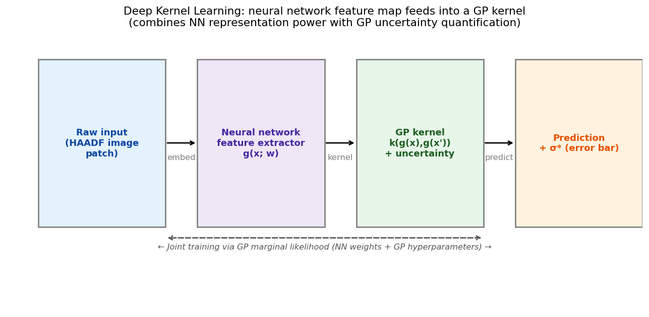
Deep Kernel Learning architecture. Raw input (HAADF image patch) is transformed by a neural network feature extractor \(g(\mathbf{x}; w)\) into a low-dimensional embedding. A base kernel (RBF) then operates in the embedded space. All parameters — NN weights and GP hyperparameters — are trained jointly by maximising the GP marginal likelihood. This combines NN representation power with GP uncertainty quantification. Wilson, Andrew G. et al., (2016)

Walk through the four boxes left to right. Box 1 (raw input): a 32×32 HAADF patch — 1024 numbers, most of which are instrument noise. Box 2 (NN): a CNN with 3–5 layers that extracts structural features — atom positions, lattice spacing, defect type — and outputs a 32- or 64-dimensional vector. Box 3 (GP kernel): RBF kernel evaluated on the 32-D embeddings. Two patches that look structurally similar will be close in embedding space and will have high kernel correlation. Box 4 (prediction): GP posterior mean (best prediction) and σ* (uncertainty) — the acquisition function is computed from these.
The “joint training via GP marginal likelihood” arrow at the bottom is the key. The likelihood gradient flows backward through the GP formulas, through the kernel, and into the NN weights. This is just standard automatic differentiation — the same backprop the students know from Week 5.
Honest caveat: DKL requires enough training data to learn a useful feature map (typically ~100 measurements minimum). For very small datasets (n < 20), the NN feature map will overfit and the GP uncertainty will be unreliable. In those cases, a hand-crafted feature (e.g. a HAADF intensity profile, a diffraction pattern scalariser) is more robust.
Transition: “DKL was applied to real 4D-STEM experiments by Roccapriore et al. 2022.”

DKL for 4D-STEM: from patch to acquisition

Input: HAADF image patches (each patch centred on a candidate probe position).
NN feature extractor: small CNN (3–5 layers) produces a 32-D embedding that captures local structural information (atom columns, defect density, grain boundary proximity).
Target (scalariser function): a scalar derived from the 4D-STEM diffraction pattern at that position — e.g., the centre-of-mass (CoM) magnitude encoding the local electric field, or the strain metric from NBED disc positions.
GP head: gives \(\mu^*\) (predicted CoM) and \(\sigma^*\) (uncertainty) at any HAADF-visible but un-probed location. The UCB acquisition function then selects the most informative position to probe next.
Payoff: the DKL model can reconstruct the CoM map from \(< 1\%\) of all pixel positions, reducing beam dose by \(\sim 30\times\) vs full-scan 4D-STEM. Roccapriore, Kevin M. et al., (2022), doi:10.1021/acsnano.1c11118

The scalariser function is the key design choice. The experimenter chooses what they care about and encodes it as a scalar reward. CoM magnitude = “I want to find where local electric fields are strongest.” Bragg disc distance = “I want to find where strain is highest.” DPC angle = “I want to map the direction of the polarisation.” The rest of the DKL pipeline is identical — only the scalariser changes.
The 1% / 30× figure is from Roccapriore et al. (ACS Nano 2022). Context: a full 4D-STEM scan of a 256×256 pixel field requires 65536 probe positions. The DKL active-learning approach achieves comparable quality with 655 positions (~3 minutes of dose vs ~90 minutes).
For beam-sensitive materials (MnPS3 in the paper), dose reduction is not a convenience — it is the difference between observing the sample intact and destroying it. The DKL approach directly saves the specimen.
Transition: “Let’s look at the experimental workflow.”

DKL: kernel network architecture

Kernel transformation: the standard GP RBF kernel \(k(\mathbf{x},\mathbf{x}')\) is replaced by \(k(g(\mathbf{x};w), g(\mathbf{x}';w))\) where \(g\) is a deep network. This is a deep kernel — the kernel itself is parameterised by the NN weights \(w\).
Training objective (intuition): all parameters — NN weights \(w\) and GP hyperparameters \(\theta\) — are trained jointly by maximising the GP marginal likelihood. The likelihood “tells” the NN which features of the input predict the target; they learn together in one pass of backpropagation. No formula needed — the machinery is identical to the Week 9 GP fit, extended to also learn the feature map.
Scalability: the base GP \(O(N^3)\) cost remains. For \(N > 500\) probe positions, use sparse GP approximations (inducing points). GPyTorch implements this with \(O(NM^2)\) cost for \(M \ll N\) inducing points.
Uncertainty inheritance: the GP head provides calibrated \(\sigma^*\) even for high-dimensional image inputs — the UCB acquisition function is directly applicable. Wilson, Andrew G. et al., (2016)

For the curious (not examined): the exact training objective is the GP log marginal likelihood \(\log p(\mathbf{y} \mid \mathbf{X}, w, \theta) \propto -\mathbf{y}^\top (K_{w,\theta} + \sigma_n^2 I)^{-1}\mathbf{y} - \log|K_{w,\theta}+\sigma_n^2 I|\). This is the same formula from Week 9, but the kernel matrix \(K_{w,\theta}\) now depends on the NN weights \(w\). Backpropagation through the marginal likelihood computes \(\partial \log p / \partial w\) and \(\partial \log p / \partial \theta\) simultaneously — two sets of gradients, one training loop.
The intuition is sufficient for this course: the NN learns features that make the GP likelihood high. The formula gives the precise mathematical content for students who want to implement DKL.
The marginal likelihood objective is the same one from Week 9 (we don’t derive it, but it appeared in the notes). The key new piece is that the kernel matrix \(K_{w,\theta}\) now depends on the NN weights \(w\). Backpropagation through the marginal likelihood computes \(\partial \log p / \partial w\) and \(\partial \log p / \partial \theta\) simultaneously — two sets of gradients, one training loop.
GPyTorch (from Caltech/CMU) is the practical library for DKL. It combines PyTorch (familiar to students from Week 5) with GP inference. DKL is built-in: gpytorch.kernels.RBFKernel(active_dims=...) wrapped around a torch.nn.Sequential feature extractor.
The inducing-point sparse GP: the \(M\) inducing points are learnable parameters (not data points). After training, \(M \approx 50\) inducing points can summarise \(N = 10^4\) probe positions. The approximate posterior is still Gaussian — UCB and EI still apply without modification.
Transition: “Automated 4D-STEM experimental results.”

Automated 4D-STEM: experimental workflow

Step 1 — HAADF pre-scan: a fast, low-dose HAADF image covers the full field of view. This image is the input to the DKL feature extractor. No full 4D-STEM acquisition yet.
Step 2 — Bootstrap: measure 4D diffraction patterns at a small random set of positions (~50). Use these to train the DKL model.
Step 3 — Active acquisition loop: (a) refit DKL; (b) compute UCB acquisition over all un-probed HAADF-visible positions; (c) move the electron probe to the top-scored position; (d) acquire the diffraction pattern; (e) update the dataset; (f) repeat.
Step 4 — Terminate and reconstruct: after budget (or convergence), predict the full-field scalariser map from the DKL posterior mean. Uncertainty map shows where the prediction is confident vs uncertain. Roccapriore, Kevin M. et al., (2022), doi:10.1021/acsnano.1c11118

The HAADF pre-scan is cheap: the HAADF detector integrates intensities, so a fast annular dark-field scan costs ~1% of the dose of a 4D-STEM scan. The pre-scan gives the feature extractor (CNN) its input everywhere in the field, even for positions never probed with the full 4D measurement.
The bootstrap step (step 2) is the cold-start solution: the DKL model needs some 4D data to initialise the GP. Without it, the uncertainty is uniform everywhere and the acquisition function is equivalent to random sampling. Typically 30–100 bootstrap positions suffice.
The loop runs autonomously — no human decides the next measurement. The microscope computer executes: (1) evaluate acquisition on GPU, (2) send stage+deflector command, (3) acquire 4D pattern, (4) append to dataset, (5) go to (1). On modern TEMs with a digital control interface (Nion, FEI API, JEOL Astra), this loop is implementable today.
Transition: “What does the output look like?”

Automated 4D-STEM: results on graphene and MnPS₃

Graphene (bilayer, twist-induced domains): DKL reconstructs the CoM magnitude map from 3% of pixel positions. The acquisition function preferentially samples near domain boundaries (highest structural variability → highest information gain). Result: sharp domain maps indistinguishable from full-scan ground truth. Roccapriore, Kevin M. et al., (2022), doi:10.1021/acsnano.1c11118
MnPS₃ (beam-sensitive van der Waals material): full 4D-STEM would cause sulfur vacancy generation. DKL achieves comparable quality with \(< 3\%\) of positions → specimen survives.
Strain mapping (NBED, Bragg disc scalariser): acquisition function prefers positions near grain boundaries (high strain gradient). DKL recovers strain maps with nanometre resolution from 15% of positions.
Key limitation: DKL assumes the scalariser function is smooth in the learned feature space. For materials with sharp phase boundaries or discontinuous properties, the GP prediction jumps — and the coverage guarantee no longer holds.

The graphene result is the “sanity check”: on a well-characterised material with a known answer, does DKL give the right answer at 3% sampling? Yes. This validates the method before applying it to unknown materials.
The MnPS3 result is the “killer application”: a material where conventional 4D-STEM physically cannot work (beam damage destroys it before the scan is complete). DKL turned a previously inaccessible experiment into a routine one.
The strain mapping result is practically important for the students’ field: strain mapping is a core 4D-STEM application in semiconductor and thin-film research. Reducing scan time by 7× means a measurement that used to take an hour now takes 8 minutes — transformative for throughput.
The key limitation note is essential: the GP is a smooth model. If the material has a sharp phase boundary that the feature extractor doesn’t capture, the GP will smooth over it and the uncertainty will be artificially low there. Always check the DKL uncertainty map for unexpectedly low uncertainty in structurally complex regions.
Transition: “So far we have talked about optimising one measurement at a time. The bigger vision is continuous automated control.”

DKL vs standard BO: when to use which

Use standard BO (GP + RBF) when: input is a scalar or low-dimensional vector (1–5 parameters); dataset has \(N < 100\) measurements; the RBF length-scale has a natural physical interpretation (e.g., length-scale in convergence angle space).
Use DKL when: input is a high-dimensional image patch or spectrum; standard GP with RBF gives poor predictions (large residuals, poorly calibrated uncertainty); you have \(N \geq 100\) bootstrap measurements to train the NN feature extractor.
Use sparse GP or inducing-point GP when: dataset grows to \(N > 500\); the \(O(N^3)\) cost becomes a bottleneck; you want real-time update during a continuous acquisition. Wilson, Andrew G. et al., (2016)
EM rule of thumb: standard BO for process parameter optimisation (1–3 parameters, 10–50 measurements); DKL for spatial field mapping (image-patch input, \(10^3\)–\(10^4\) positions); sparse GP for streaming tomographic data.

The three-way split (standard BO / DKL / sparse GP) is a practical decision guide for the students’ miniprojects. The most common mistake is applying DKL to a 3-measurement dataset — the NN feature map immediately overfits and the GP uncertainty is meaningless.
The N ≥ 100 threshold for DKL is conservative. Some papers report good DKL results from N = 50 bootstrap measurements. But for safety (especially on a miniproject with no time to debug), 100 is the recommended minimum.
The “streaming tomographic data” case for sparse GP: tilt-series tomography acquires one 2-D projection per tilt angle. After 60 tilts, \(N = 60\) — small enough for standard GP. But if each projection is a spectrum image with \(10^4\) pixels, and you want a GP over the full reconstruction space, sparse GP is needed.
Transition: “Having seen the components — BO, DKL — now the bigger picture: continuous autonomous control.”

Physics-driven autonomous experiment design

The key insight from Roccapriore et al. Roccapriore, Kevin M. et al., (2022), doi:10.1002/advs.202203422: the scalariser function encodes the physics the experimenter cares about. “Find the region of maximum local electric field” is a physics goal encoded as scalariser = CoM_magnitude. The DKL + BO system then pursues that goal autonomously.
Structure–property learning: the DKL model learns the statistical relationship between HAADF image structure and the target property (CoM, strain, plasmon energy). This relationship is itself a scientific finding — it reveals which structural features predict the measured physical response.
Nanoplasmonic discovery: the same DKL approach found bulk- and edge-plasmon-active regions in MnPS₃ autonomously — a measurement that would have taken days of manual scanning was accomplished in hours.
The vision: an operator defines the scientific objective; the instrument autonomously acquires, analyses, and reports the regions of highest interest — without human involvement in the loop.

The “physics goal as scalariser” framing is the deepest conceptual contribution of this line of work. It transforms the BO/DKL problem from “optimise an arbitrary function” to “pursue a specific scientific hypothesis.” The scalariser is a formalization of the experimenter’s prior knowledge.
Structure–property learning as a by-product: the DKL model’s learned feature space is not just a technical artifact — it is a quantitative map of which local structural motifs predict the target physical response. In a HAADF/CoM experiment, visualising which HAADF patch features have the highest gradient in the learned embedding reveals the structural driver of the electric field. This is interpretable science, not just optimization.
The nanoplasmonic result: in MnPS₃, the edge plasmon mode had been theoretically predicted but never directly imaged. The DKL acquisition function sought regions with unusual EELS spectra (high-uncertainty, high-predicted-interest) and found the edge mode without the operator knowing where to look. The autonomous system discovered the edge mode on its own.
Transition: “From BO to full closed-loop control.”

Automation as closed-loop control

The manual bottleneck: a skilled TEM operator adjusts focus, astigmatism, beam alignment, and sample drift correction in real time — using their eyes as the sensor and their hands as the actuator. This limits throughput and introduces operator-to-operator variability.
The control-loop view: every manual adjustment is a feedback loop: (1) sense the current state (image quality, beam shape); (2) compute the correction signal; (3) actuate (adjust lens current, deflector voltages); (4) repeat.
Sensors in a modern TEM: HAADF detector (image), EELS spectrometer (spectrum), 4D detector (diffraction), beam-current monitor, stage encoder (position). Together they give a high-dimensional state vector \(\mathbf{s}_t\).
Actuators: objective lens current, stigmator voltages (4 axes), scan deflectors (2D), stage motors (x,y,z,tilt), condenser aperture motor. A modern TEM has 20–50 independent actuators.

The “manual bottleneck” is real: the best TEM operators in the world can achieve ~1 nm focus stability manually; automated systems routinely achieve < 0.1 nm. The limiting factor in manual operation is human reaction time (~200 ms) and fatigue; automated systems can cycle at ~10 Hz.
Draw the control loop on the board: Sensor → State → Compute → Action → Microscope → (new) State. This is the same feedback loop students know from a thermostat — except the “thermostat” has 50 actuators and the “sensor” is a 1024×1024 diffraction pattern.
The key new idea: we replace the human operator’s intuition with a learned policy — a function that takes the current state and returns the appropriate action. The learning problem is: how do we train that policy without a human providing labels for every state?
Transition: “The answer is reinforcement learning.”

Sensors, actuators, and the state space

State \(\mathbf{s}_t\): what the microscope “knows” at time \(t\). Typically: the current image (or a feature vector from it), the current stage position, and recent calibration values.
Action \(a_t\): what the controller “does.” Discrete: move stage by ±Δx; continuous: increment lens current by δI.
The control challenge: the mapping from action to observable effect is nonlinear (magnetic lens saturation), hysteretic (remanent magnetisation), and high-dimensional (50 coupled axes). Classical PID control handles single-axis, linear systems. Machine learning is needed for coupled, nonlinear, high-dimensional cases.
BO as a special case: the BO loop from earlier is a control loop where the “action” is “choose next probe position” and the “reward” is the diffraction pattern scalariser at that position. BO is stateless — it does not use the history of actions, only the set of observations.

The hysteresis point deserves emphasis. A magnetic lens has memory: if you increase the current to 1000 mA and then reduce it to 500 mA, you get a different focal length than if you had started at 500 mA directly. This makes simple feedforward control (apply the “right” current for focus = 2 nm) unreliable. The lens’s history must be taken into account — either by always approaching focus from the same direction or by learning the hysteresis curve.
The 50 coupled axes point: stigmators, deflectors, and lenses interact. Adjusting the objective lens current shifts the beam by a small amount (lens coupling). Adjusting the stigmator changes the beam astigmatism but also its position slightly. A naive single-axis control loop that ignores coupling can oscillate. Learning the full coupling matrix is a regression problem.
BO vs RL contrast: BO is a batch-update optimiser (refit GP after each measurement). RL is an online learner (update policy after each step). For real-time control (focus correction every 100 ms), RL is more appropriate. For slower optimisation (finding the best process parameter, one measurement per hour), BO is more appropriate.
Transition: “RL gives the formal framework for the learning-based control.”

From BO to RL: two regimes of automated EM

Slow loop (BO regime): one measurement per 20 min–8 h. Example: optimise a synthesis temperature, a beam voltage, or a composition. The GP can be refitted offline; the experimenter can intervene between measurements. Best tool: Bayesian optimisation.
Fast loop (RL regime): one correction per 0.1–10 s. Example: autofocus, beam stigmation correction, drift compensation. The state changes faster than a human can respond. Best tool: reinforcement learning with a trained policy.
Bridging the gap: some tasks live in between — e.g., adapting the scan strategy during a 1-hour 4D-STEM session. DKL active learning is the bridge: it reruns the acquisition decision every ~2 s (GPU evaluation), adapting faster than BO but slower than pure RL.
Common thread: all three (BO, DKL active learning, RL) replace human intuition with a learned function that maps observations to actions. The difference is only the time scale and the learning algorithm.

The two-regime framing is a practical guide for students thinking about their own projects. If your experiment takes more than 1 minute per evaluation, use BO. If it needs correction faster than you can react, use RL. If it’s in between, use DKL active learning.
The “common thread” sentence is the conceptual synthesis. Students who understand this sentence understand the whole lecture: BO, DKL, and RL are all instances of the same idea — replace human intuition with a learned function. The machinery differs; the principle is the same.
RL in continuous control: for autofocus, the policy is typically a CNN that maps a 256×256 image to a scalar defocus correction. Training: generate synthetic training data by applying known defocus offsets to sharp reference images; train the CNN to predict the applied offset from the blurry input. The trained policy runs in ~10 ms per frame — fast enough for real-time control at 30 fps.
Transition: “Now the RL framework formally.”

Reinforcement learning: the formal framework

Agent: the learning controller — a neural network (or other model) that maps observations to actions.
Environment: the external system being controlled — the electron microscope (in our case) or the scanning stage, beam, or full instrument.
State \(s\): a description of the current situation (current image, beam properties, stage position).
Action \(a\): what the agent does at each step (set a lens current, move the stage, adjust the deflector).
Reward \(r\): a scalar signal indicating how good the current action was. The agent learns to maximise the cumulative discounted reward \(R = \sum_t \gamma^t r_t\) where \(\gamma \in [0,1)\) is the discount factor.
Policy \(\pi(a \mid s)\): the agent’s strategy — a distribution over actions given the current state. Learning a policy from rewards alone (no labels) is the RL problem. Bishop, Christopher M., (2006)

RL in one sentence: “trial and error, guided by a reward signal.” The agent doesn’t know the rules in advance; it discovers them by exploring the environment and receiving rewards for good behaviour.
The discount factor \(\gamma\): it balances immediate vs future reward. \(\gamma=0\): only the immediate reward matters (greedy). \(\gamma=0.99\): rewards 100 steps in the future are discounted by only \(0.99^{100} \approx 0.37\) — still significant. For focus control, immediate rewards (get the image sharp now) dominate and \(\gamma=0.9\) is sufficient. For long-horizon experiments (find a specific grain over a 12-hour session), high \(\gamma\) is needed.
The “no labels” point is the key differentiator from supervised learning. In supervised EM (Week 6 CNN), we needed humans to draw segmentation masks. In RL autofocus, the reward (image sharpness) is automatically computable from the image — no human annotation required. This is why RL is potentially scalable to 24/7 automated operation.
Transition: “Show the RL loop for the microscope.”

The RL control loop for the electron microscope

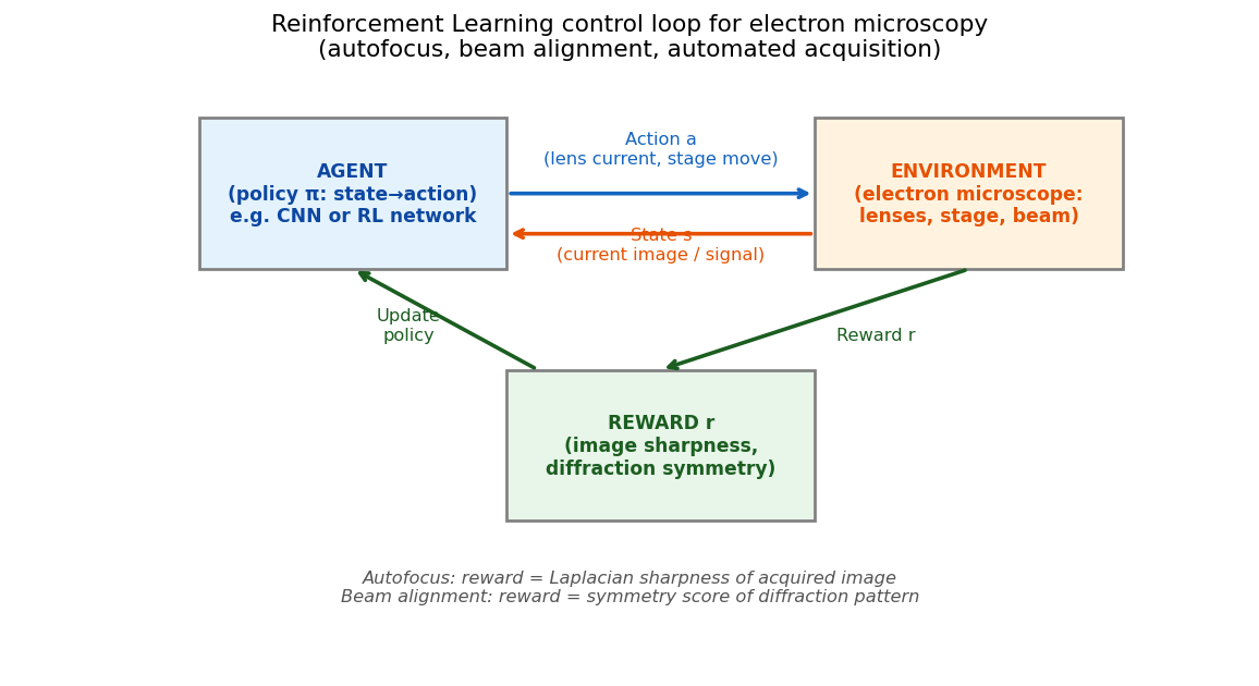
RL control loop for an electron microscope. The agent (policy network) observes the current state (image or beam measurement), selects an action (lens current change, stage move), and receives a scalar reward from the environment (the microscope). The reward signal encodes the experimental objective: sharp image (autofocus), symmetric diffraction (beam alignment), or maximum CoM magnitude (4D-STEM discovery). The policy is trained to maximise cumulative reward — no manual labels required.

Walk through the figure. The central loop: state (current image) → agent (policy π) → action (lens current) → environment (microscope hardware) → new state + reward. The reward signal connects the microscope output back to the policy update.
Emphasise: the policy is a neural network trained by gradient descent on the cumulative reward signal. The gradient of the reward with respect to the policy weights is the key computation — this is the policy gradient algorithm. We are not deriving it today (that is a full RL course), but the students should know it exists and works.
The three reward examples in the figure correspond to three real applications: autofocus (next slide), beam alignment (following slide), and BO-guided 4D-STEM (earlier today). All three use the same RL framework; only the reward function and action space differ.
Transition: “The simplest and most practical case: autofocus.”

RL policy gradient: how the agent learns (intuition)

The learning objective: maximise \(J(\pi) = \mathbb{E}_\pi[\sum_t \gamma^t r_t]\) — expected cumulative discounted reward under policy \(\pi\).
Intuition: if a sequence of actions led to high return, increase the probability of those actions. If it led to low return, decrease it. This is trial-and-error learning, formalised as gradient ascent on expected reward — no labels required.
How it works (conceptual): the policy is a differentiable function (e.g. a CNN). The gradient of the expected reward with respect to the policy parameters is estimated from observed episodes. Backprop through the policy updates its weights in the direction of higher reward.
Not examined for this course: the mathematical derivation (policy gradient theorem). The conceptual points — (1) RL learns from rewards, no labels; (2) gradient ascent on expected return; (3) the same backprop the students know from Week 5 — are all that is required. Bishop, Christopher M., (2006)

For the curious (not examined): the policy gradient theorem is \(\nabla_\pi J = \mathbb{E}_\pi\!\left[\sum_t \nabla_\pi \log\pi(a_t|s_t) \cdot G_t\right]\) where \(G_t = \sum_{k \geq t} \gamma^{k-t} r_k\) is the return from step \(t\). This is the REINFORCE estimator. It is unbiased but high-variance; modern algorithms (PPO, TRPO) add variance-reduction tricks. The formula is the theoretical backbone of RL (REINFORCE algorithm, PPO, A3C) but the students are not expected to derive or implement it.
The policy gradient theorem is the theoretical backbone of modern RL (REINFORCE algorithm, PPO, A3C). We present it for completeness but the students are not expected to derive or implement it. The key phrase: “if an action led to good outcomes, do it more; if it led to bad outcomes, do it less.”
The analogy to supervised learning: in supervised learning, the loss function is MSE or cross-entropy — both have clean gradients. In RL, the “loss” is the negative expected return, and the gradient involves the policy log-probability weighted by the observed return. This is the REINFORCE gradient estimator. It is unbiased but high-variance — modern algorithms (PPO, TRPO) add variance-reduction tricks.
For autofocus RL specifically: the policy is a CNN. The action is the defocus correction. The reward is the sharpness of the next image. One RL “episode” = one autofocus correction cycle (start blurry, correct, end sharp). Training: run thousands of simulated episodes on synthetic blurry images; update the CNN policy after each episode.
Transition: “Apply this to autofocus.”

RL key concepts: comparison table

Concept	Supervised learning	RL for EM control
Input	Image, spectrum	State \(s_t\) (current image)
Output	Label, regression value	Action \(a_t\) (lens Δ-current)
Training signal	Human labels \(y_i\)	Reward \(r_t\) (sharpness score)
Learning	Minimise loss	Maximise cumulative reward
Data	Fixed labelled dataset	Online interaction with microscope
Labels needed	Yes (expensive)	No (reward is computed automatically)

The key advantage of RL for microscopy control: the reward function is automatically computable from the microscope output — no human annotation loop is needed. Bishop, Christopher M., (2006)

Walk through the table row by row. The most important contrast: “Labels needed: Yes vs No.” This is why RL is attractive for 24/7 automated operation — once the policy is trained (on simulations), it can operate the microscope indefinitely without human intervention.
The “online interaction” row is also key. Supervised learning trains on a fixed, pre-collected dataset. RL learns while interacting — every microsecond of autonomous operation generates new training data. An RL autofocus policy improves as it runs, in principle.
The caveat on “improves as it runs”: online RL can also forget (catastrophic forgetting) or diverge (reward hacking). In practice, production systems use a fixed trained policy (trained offline on simulations) rather than a continuously updating online policy. The continuous improvement happens only in research settings with careful safety guards.
Transition: “Autofocus and beam alignment: the two most common RL applications in EM.”

RL for autofocus: learning to maximise image sharpness

State: the current image (or a feature vector derived from it: Laplacian variance, FFT high-frequency power).
Action: change the objective lens defocus by \(\pm\Delta f\) (discrete: ±0.5 µm, ±2 µm, ±5 µm) or continuously.
Reward: image sharpness index. Most common: Laplacian variance \(r = \frac{1}{N}\sum_{i,j} (\nabla^2 I)_{ij}^2\). Also used: sum of squared high-frequency FFT components \(r = \|\hat I(\mathbf{k})\|^2_{\mathbf{k} : |\mathbf{k}|>k_0}\).
Why RL beats sweep-and-search: traditional autofocus sweeps defocus through 10–20 values and picks the maximum. With an RL policy, the agent directly predicts the correct defocus from a single blurry image — one step, not a sweep. Speed: 100× faster.

The Laplacian variance is zero for a perfectly blurred (constant) image and maximum for a perfectly sharp image. It is computable in milliseconds on a GPU. The FFT variant is equivalent but emphasises specific spatial frequencies — useful if the sample has known periodicity (crystal lattice fringes).
The “one step vs sweep” distinction is important for beam-sensitive samples. A traditional sweep exposes the sample to 10–20 frames before achieving focus; an RL policy uses 1 frame. For MnPS3 (dose budget = 3 frames before damage), a sweep is simply not possible — RL autofocus is the only viable approach.
RL training for autofocus: generate synthetic training data by applying known defocus offsets to sharp reference images, then optimise the policy to predict (and correct) the applied offset. No real EM samples needed for training — transfer to real images is straightforward.
Transition: “Show the reward landscape.”

Autofocus as RL: the reward landscape

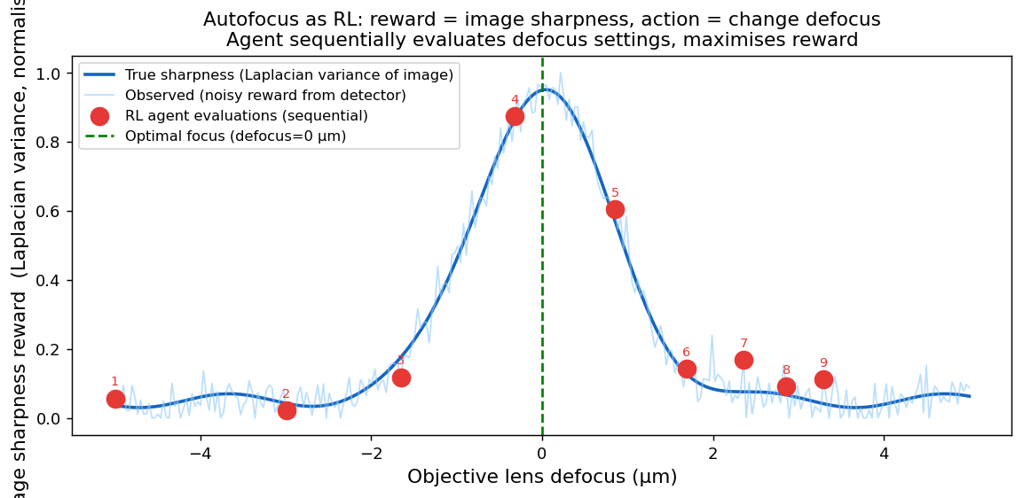
Image sharpness reward (Laplacian variance, normalised) as a function of objective lens defocus (µm). The true sharpness (blue) peaks sharply at 0 µm — the in-focus position. The noisy observed reward (light blue) is what the RL agent sees at each step. The RL agent’s sequential defocus evaluations (red dots, numbered) converge to within ±0.1 µm of the optimum in fewer than 9 steps — faster than a traditional 20-point sweep and without exposing the sample to unnecessary dose.

Walk through the figure. The blue curve is the noiseless sharpness as a function of defocus — it is a sharp peak (width ~1 µm) centred at zero. The light blue curve is what the RL agent actually observes (camera noise, vibration, sample drift add noise to each measurement).
The red numbered dots show the agent’s exploration trajectory. It starts at a large defocus (dot 1), quickly identifies the peak region (dots 4–6), then refines near the optimum (dots 7–9). This is similar to the BO trajectory seen earlier — and that is not a coincidence: autofocus is a 1-D BO problem when framed this way.
The key difference from BO: in autofocus, the agent can change the state (set a new defocus) and immediately observe the reward. In BO for process parameters, each “evaluation” is a full EM experiment (hours). The real-time nature of autofocus allows online RL with fast feedback; the slow nature of process optimisation requires sample-efficient BO.
Transition: “Beam alignment uses a different reward: diffraction symmetry.”

Beam alignment via diffraction symmetry

The alignment problem: the electron beam must travel through the optical axis of every lens for optimal image quality. Tilt, shift, and astigmatism cause the beam to deviate — producing elongated diffraction spots and asymmetric diffraction patterns.
The diffraction symmetry reward: a centrosymmetric crystal with a perfectly aligned beam produces a diffraction pattern with \(m\)-fold rotational symmetry. The reward is a symmetry score: high when the pattern is more symmetric.
Action space: beam tilt \((\Delta\theta_x, \Delta\theta_y)\) and shift \((\Delta x, \Delta y)\) in four-dimensional combined action space.
RL advantage over manual: manual alignment requires an experienced operator to interpret diffraction patterns and know which control to adjust. The RL policy learns the causal chain automatically from the reward signal — it can run while the operator is absent. Roccapriore, Kevin M. et al., (2022), doi:10.1002/advs.202203422

The rotational symmetry score is computable in milliseconds from any diffraction pattern. For a 4-fold symmetric lattice (e.g. Si [001] zone axis), the score compares \(I(k_x, k_y)\) with \(I(-k_x, k_y)\), \(I(k_x, -k_y)\), \(I(-k_x, -k_y)\). Perfect 4-fold symmetry = maximum score; any beam tilt breaks the symmetry and reduces it.
The four-dimensional action space (tilt x, tilt y, shift x, shift y) is not trivially navigable by a human. The RL agent learns the joint sensitivity: increasing tilt_x also shifts the beam pattern, requiring a compensating shift_x. The agent learns this coupling from the reward feedback — no manual calibration required.
The safety constraint: during alignment, the beam may briefly pass through a region of the sample that is not the intended region of interest. RL policies for alignment should include a “beam protection” constraint: never tilt more than ±5 mrad from the starting position without rechecking the stage position. This is a standard constraint in modern TEM control software.
Transition: “Having seen the components — BO, DKL, RL — what is the vision for the fully autonomous lab?”

Autofocus + alignment: the combined control hierarchy

Level 1 — Real-time correction (< 100 ms): autofocus (RL policy, one image → one defocus command), stigmation correction (RL), drift compensation (RL or Kalman filter). These run continuously, invisibly to the operator.
Level 2 — Session-level optimisation (minutes): beam alignment (RL), aperture centering (rule-based or RL), gun tilt optimisation (RL). Run once per microscope session or after each sample change.
Level 3 — Experiment-level optimisation (hours): acquisition parameter optimisation (BO), sample-position selection (DKL active learning). Run once per scientific objective.
Hierarchy as a system: the three levels interact. Level 1 keeps the instrument stable so Level 3’s BO measurements are comparable. Level 3’s BO-chosen parameters are passed to Level 1 as setpoints. Together they constitute a fully autonomous EM experiment pipeline.

The three-level hierarchy is not hypothetical — it describes how modern commercial TEMs (e.g., Thermo Fisher Velox, Gatan DigitalMicrograph with AutoTuning) actually work. Level 1 is already automated in all modern instruments. Level 2 (beam alignment RL) is available in research software. Level 3 (BO for experiment design) is the research frontier.
The “invisible to the operator” point for Level 1 is important for context: students who have used a modern TEM have already experienced automated control — they just may not have known it was there. The autofocus button in software is an RL (or classical) policy, not a human knob.
The interaction between levels is the key systems insight. If Level 1 (autofocus) fails silently, Level 3 (BO) will measure noisy, blurry images and the GP surrogate will be misleading. A robust autonomous system monitors all three levels and raises alerts if Level 1 fails to converge.
Transition: “The full vision — and its limits.”

The autonomous-lab vision: limits and honest risks

The promise: a self-driving TEM runs 24/7. The operator defines an objective (“find all Ni₃Al precipitates and measure their size distribution”). The instrument acquires, analyses, and reports without human intervention. Roccapriore, Kevin M. et al., (2022), doi:10.1002/advs.202203422
What works today: autofocus (RL, production-deployed), beam stigmation correction (RL, deployed on some systems), single-parameter BO experiments (e.g., optimise annealing temperature, run in 1–2 day loops).
Current limits: (1) reward hacking — an agent maximising Laplacian sharpness can produce “sharp” images of noise or contamination; careful reward design is essential. (2) Sim-to-real gap — policies trained on simulated EM images fail on real specimens with unexpected contrast mechanisms. (3) Multi-step long-horizon tasks — finding a rare defect across a 1 mm² sample area requires hierarchical RL that is not yet production-ready.
Ethical and epistemic risks: autonomous decisions about where not to measure can introduce systematic bias. Always archive the full trajectory of where the autonomous agent chose to measure — and where it did not.

The “what works today” list is deliberately conservative. Students should distinguish between deployed systems (autofocus: yes, on every modern TEM with auto-alignment software) and research prototypes (DKL 4D-STEM: demonstrated in papers, not yet in vendor software). The gap matters for their PhD projects.
Reward hacking is the deepest problem. A famous RL example: an agent trained to maximise speed in a racing game learned to spin in circles because the speedometer kept registering high speed. In EM: an autofocus agent trained to maximise Laplacian variance might tilt the beam to create artificial edge contrast. Always test the policy on out-of-distribution images before deployment.
The “archive the trajectory” point is a scientific integrity issue. If an autonomous agent skipped a region of a sample because its acquisition function scored it low, and that region contained the most interesting defect, the published result is misleading. Full transparency about the autonomous acquisition trajectory is required for reproducibility.
The forward link to Week 11: “The autonomous acquisition collects data. But we haven’t yet asked: given the data, what is the underlying structure? That is the inverse problem — the topic of the next two weeks.”

Forward link: Week 11 — Imaging inverse problems I

Today’s output: a set of measurements \(\{(x_i, y_i)\}\) acquired by an autonomous BO or RL agent — maximally informative, minimally dosed.
Week 11’s question: given those measurements, how do we reconstruct the underlying physical quantity? An EELS spectrum map tells us elemental composition. A 4D-STEM dataset encodes local electric fields. A tilt series encodes the 3-D structure. None of these are directly the quantity we want — they require inversion.
The mathematical framework: imaging is a forward model \(y = \mathcal{A}(x) + \epsilon\) where \(\mathcal{A}\) is the measurement operator (e.g., a matrix, a Fourier transform, a simulation). Recovering \(x\) from \(y\) is an ill-posed inverse problem — many \(x\) are consistent with the observations.
The GP connection: the uncertainty-guided sampling of this week ensures that the measurements \(\{y_i\}\) are maximally informative for the inverse problem of next week. Active learning and inverse problems are two sides of the same coin.

Close the arc: Week 9 gave uncertainty. Week 10 turned uncertainty into action (BO and RL). Week 11 will use the collected data to reconstruct structure. The three weeks form a complete loop: sense → plan → infer → sense again.
The “two sides of the same coin” framing: the GP posterior from Week 9 is both the decision-maker (this week: where to measure) and the prior for the inversion (next week: what does the data tell us about the structure). Some EM reconstruction algorithms (phase retrieval, STEM-EELS) explicitly use GP priors on the structure.
Practical note for students doing the miniproject: if your project involves EM data acquisition AND reconstruction, the natural pipeline is: use BO to choose acquisition parameters → collect data at those parameters → invert (Week 11 methods) → report the reconstructed structure with GP-derived uncertainty. That is a complete, honest, examinable data-science workflow.
Mention the notebook: “The Week 10 notebook gives you the BO loop. Week 11’s notebook will give you the inversion. Together they are the data-science stack.”

Continue

→ Next: Week 11 — Imaging inverse problems I
← Back: Week 09 — Probability, uncertainty & Gaussian processes
All courses

References

Taking the human out of the loop: A review of Bayesian optimization, Proceedings of the IEEE, Bobak Shahriari, Kevin Swersky, Ziyu Wang, Ryan P. Adams, & Nando de Freitas.

Gaussian processes for machine learning, Carl Edward Rasmussen & Christopher K. I. Williams.

Deep kernel learning, Proceedings of the 19th international conference on artificial intelligence and statistics (AISTATS), Andrew G. Wilson, Zhiting Hu, Ruslan Salakhutdinov, & Eric P. Xing.

Automated experiment in 4D-STEM: Exploring emergent physics and structural behaviors, ACS Nano, Kevin M. Roccapriore, Ondrej Dyck, Mark P. Oxley, Maxim Ziatdinov, & Sergei V. Kalinin https://doi.org/10.1021/acsnano.1c11118.

Physics discovery in nanoplasmonic systems via autonomous experiments in scanning transmission electron microscopy, Advanced Science, Kevin M. Roccapriore, Sergei V. Kalinin, & Maxim Ziatdinov https://doi.org/10.1002/advs.202203422.

Pattern recognition and machine learning, Christopher M. Bishop.

Data Science for Electron Microscopy Week 10: Active & automated electron microscopy