Mathematical Foundations of AI & ML
Unit 10: Attention & Transformers


Before transformers: Recurrent Neural Networks
The sequence problem:
- CNNs fail on sequences — no notion of “time” or “long-range” order.
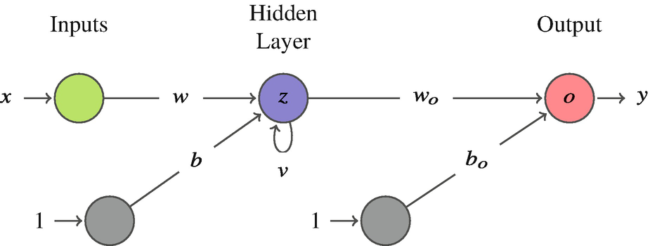
- RNNs added a recurrent loop: the output of a neuron feeds back as its own input at the next time step.
- The network state \(z_t\) carries a “memory” of the past.
- Used for time series, speech, NLP throughout the 2010s.
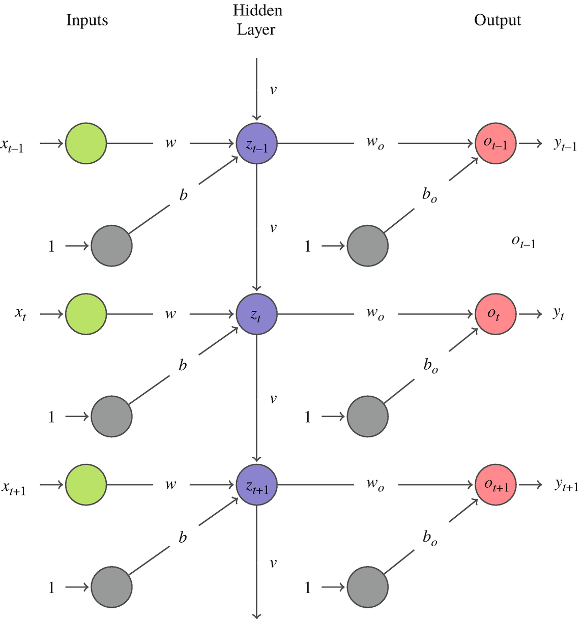
RNNs unrolled through time
“Unrolling” repeats the RNN block for each step — a chain \(z_0 \to z_1 \to \cdots \to z_T\) with the same recurrent weight \(v\) reused every step.
- Backprop to an early weight multiplies the recurrent Jacobian once per step:
\[ \frac{\partial \mathcal{L}}{\partial \theta}\;\propto\;\prod_{t=1}^{T}\frac{\partial z_t}{\partial z_{t-1}}\;\sim\;v^{\,T} \]
- \(|v|<1 \;\Rightarrow\; v^{T}\to 0\) — vanishing gradient: early steps stop learning.
- \(|v|>1 \;\Rightarrow\; v^{T}\to \infty\) — exploding gradient.
- Exactly the product-of-Jacobians mechanism from Unit 6 — you have seen this failure mode before; it is not new.
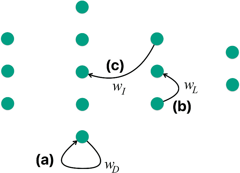
Types of feedback in recurrent networks
- (a) Direct feedback: output of a neuron feeds back to itself — the basic RNN loop.
- (b) Lateral feedback: output of a neuron feeds into a neighbor in the same layer.
- (c) Indirect feedback: output of a neuron feeds into a layer upstream.
- Each type enables different memory structures.
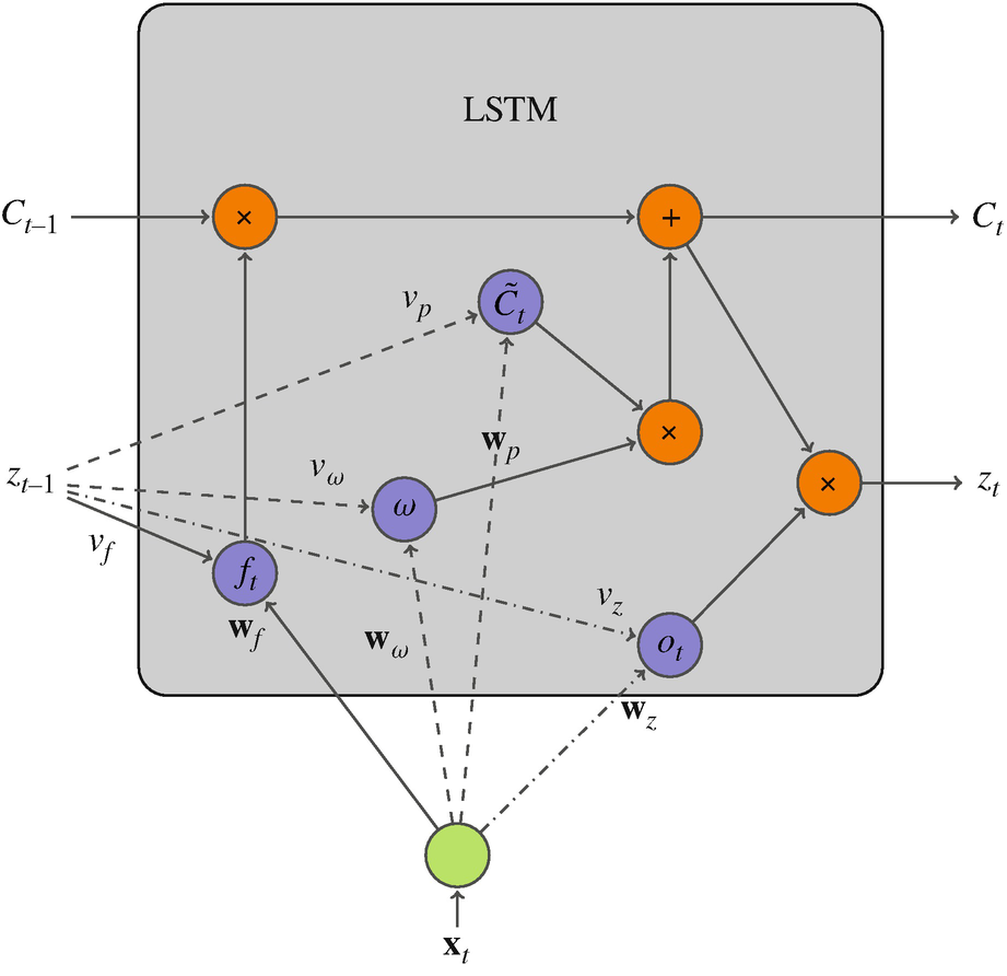
Long Short-Term Memory (LSTM)
LSTM adds a separate “state” track \(C_t\) — a long-term memory highway:
- Forget gate: decides what fraction of the old state \(C_{t-1}\) to keep (\(f_t \in [0,1]\)).
- Input gate: proposes a new state \(\tilde C_t\) and a weight \(\omega\) for how much to add.
- Output gate: produces \(z_t\) by applying an activation to the new state.
- The state \(C_t\) flows with additive updates — gradients no longer vanish exponentially.
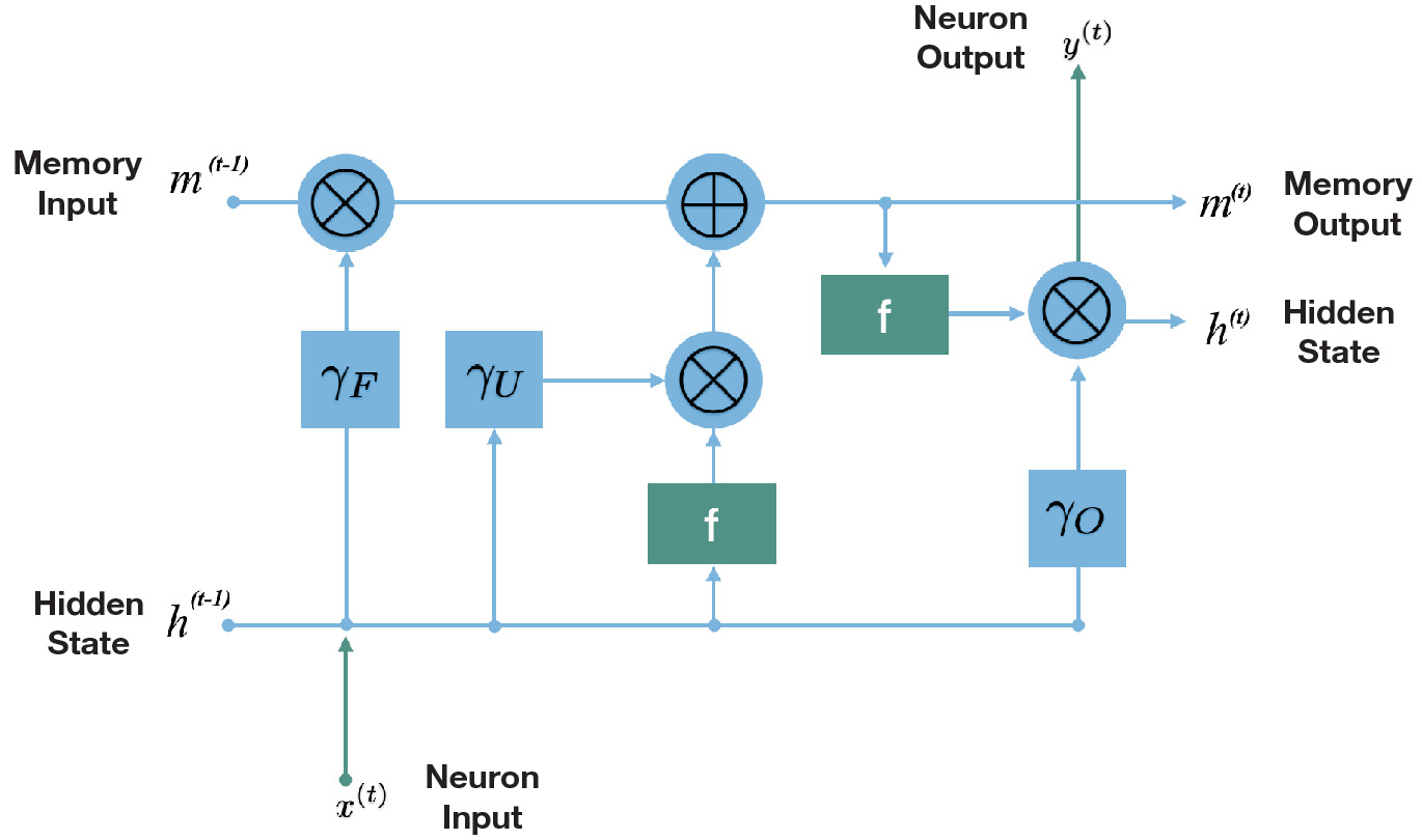
LSTM signal flow (gate view)
- At each time step, two quantities flow forward: the memory \(m\) (state) and the hidden state \(h\).
- The three gates (forget, update, output) act as learned valves on this flow.
- The forget gate clears irrelevant history; the update gate writes new information; the output gate reads the result.
- LSTMs dominated NLP benchmarks from ~2014 to 2017.
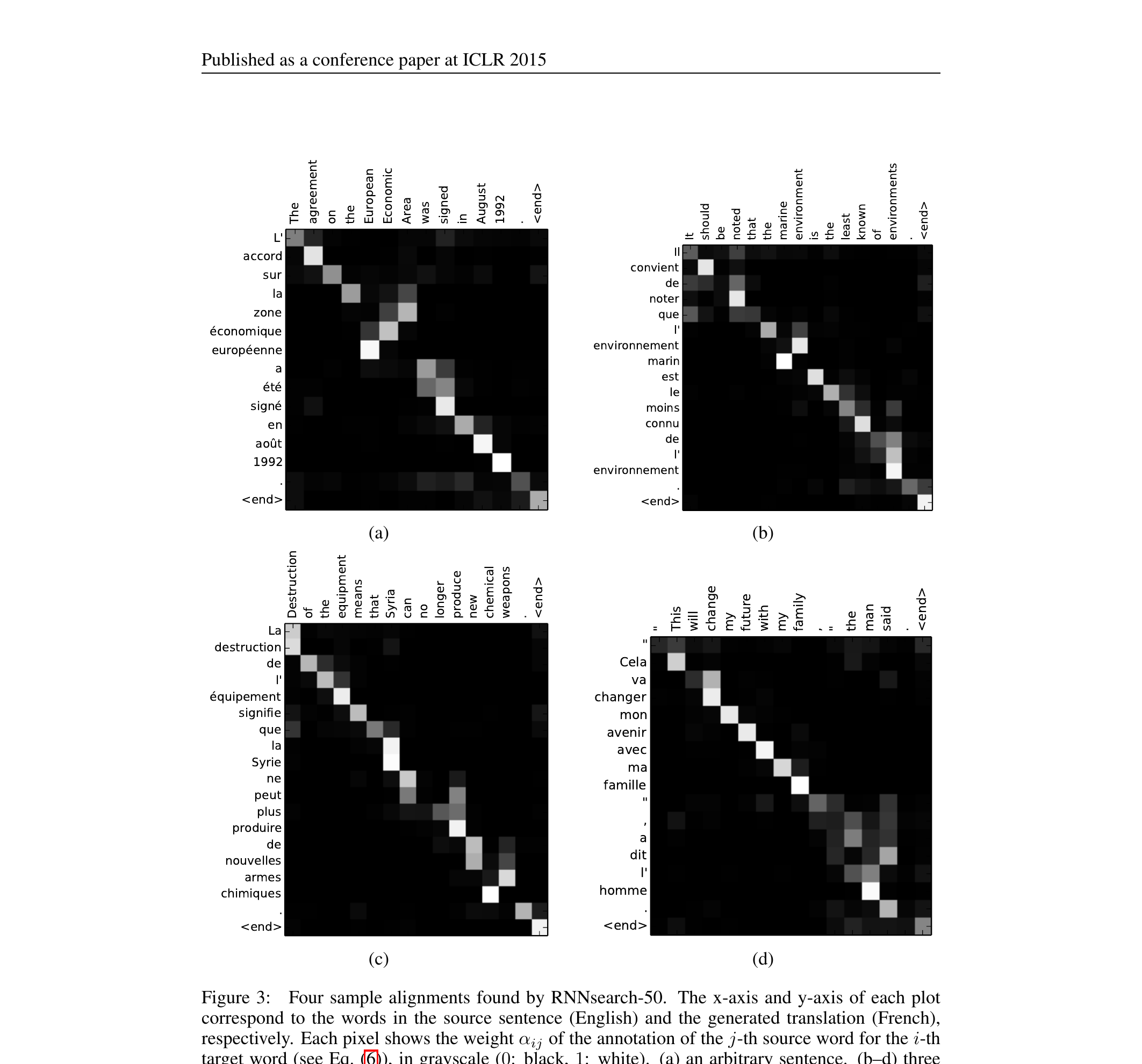
What does the attention matrix tell us?
- \(\mathrm{softmax}(S) \in \mathbb{R}^{n \times n}\): each row sums to 1.
- Entry \((i, j)\) is “how much position \(i\) pays attention to position \(j\).”
- Visualizing this matrix is one of the most useful interpretability tools in modern ML.
- For a ViT classifying a defect: the attention map shows which image patches the model used.
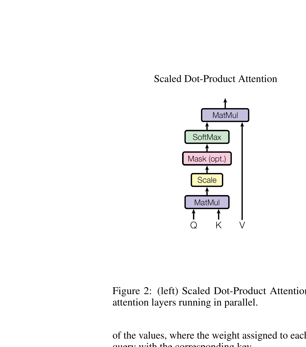
The scaled dot-product formula
The full self-attention layer:
\[ \boxed{\,\mathrm{Attention}(Q, K, V) = \mathrm{softmax}\!\left(\frac{QK^T}{\sqrt{d_k}}\right) V.\,} \]
The only difference from what we just derived: the scaling factor \(\sqrt{d_k}\).
Why \(\sqrt{d_k}\)?
- Without scaling: as \(d_k\) grows, \(q_i^T k_j\) has variance proportional to \(d_k\) (sum of \(d_k\) products).
- Large variance scores → softmax saturates → gradients vanish on most entries.
- Dividing by \(\sqrt{d_k}\) keeps the variance constant, so the softmax stays in its responsive range.
- For typical \(d_k = 64\): divide by 8. Small detail, big effect on training.
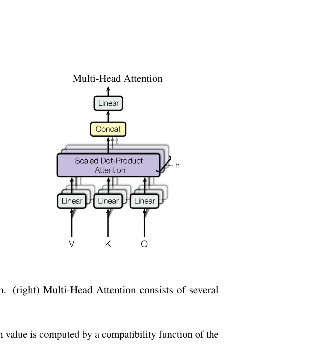
Multi-head attention — definition
For each head \(i = 1, \ldots, h\):
\[ \mathrm{head}_i = \mathrm{Attention}(Q W_i^Q, K W_i^K, V W_i^V), \]
with each head’s projection matrices independent. Concatenate and project:
\[ \mathrm{MultiHead}(Q, K, V) = \mathrm{Concat}(\mathrm{head}_1, \ldots, \mathrm{head}_h) W^O. \]
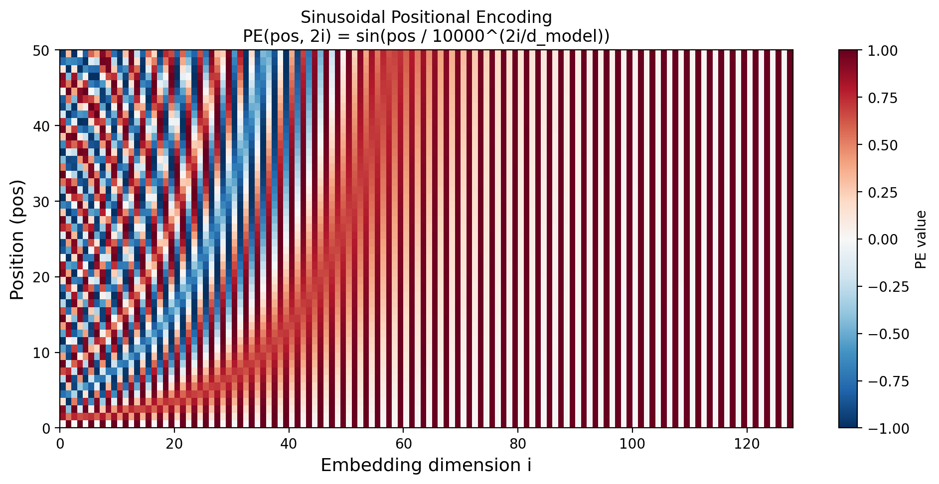
Sinusoidal positional encoding
For position \(\mathrm{pos}\) and embedding dimension \(i\):
\[ \mathrm{PE}(\mathrm{pos}, 2i) = \sin(\mathrm{pos} / 10000^{2i/d_{\text{model}}}), \] \[ \mathrm{PE}(\mathrm{pos}, 2i+1) = \cos(\mathrm{pos} / 10000^{2i/d_{\text{model}}}). \]
Add \(\mathrm{PE}\) to the token embeddings before the first attention layer: \(\tilde x_i = x_i + \mathrm{PE}(i, \cdot)\).
Sinusoidal positional encoding matrix for 50 positions and 128 dimensions. Low dimensions oscillate rapidly (fine-grained position); high dimensions change slowly (coarse-grained). Each row is a unique positional fingerprint.
The transformer block
   x  ──┐
        ├─► LayerNorm ─► Multi-Head Attn ──► (+) ─►
        └────────────────────────────────────┘   │
                                                 │
        ┌────────────────────────────────────────┘
        │
        ├─► LayerNorm ─► MLP (2-layer FF) ─────► (+) ─► output
        └─────────────────────────────────────────┘
Two sublayers: attention (mixes positions) and MLP (transforms each position independently). Each wrapped in a residual connection and LayerNorm.
![]()
Cross-attention (briefly)
- In encoder-decoder, the decoder’s middle sublayer is cross-attention: queries from the decoder, keys and values from the encoder.
- “Each decoder position decides what to pull from the encoder representation.”
- Used in image captioning, translation, and conditional generation
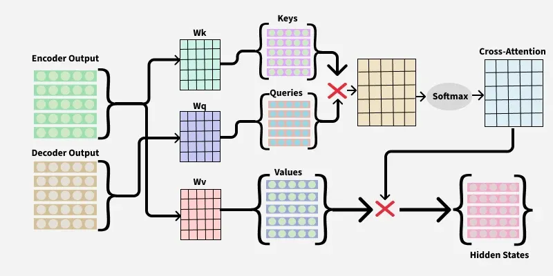
Cross-attention in encoder-decoder transformer. Queries from decoder, keys and values from encoder. Each decoder position decides what to pull from the encoder representation. (Vaswani et al. 2017, fig. 3).
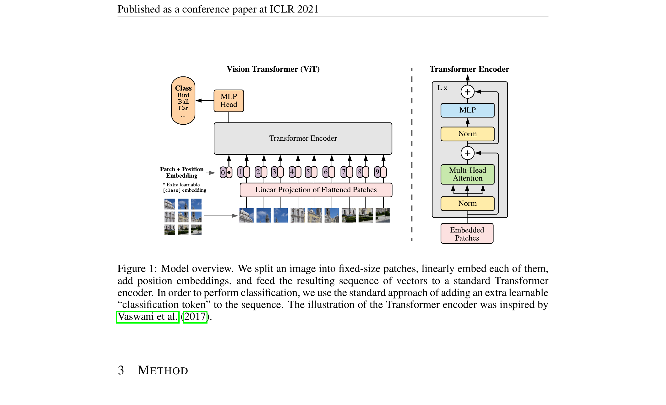
Vision Transformer (ViT)
- Take an image. Split it into a grid of fixed-size patches (e.g., 16×16 pixels).
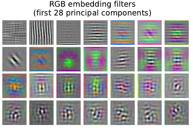
- Flatten each patch to a vector. Apply a learned linear projection to get a token embedding.
- The image is now a sequence of patch tokens. Add positional embeddings.
- Apply a standard transformer encoder. Use the output of a special [CLS] token as the image representation.
That’s it. ViT is “transformer on patches.” No convolutions, no spatial inductive bias.
ViT — patch embedding
For a \(224 \times 224\) image with \(16 \times 16\) patches:
- Number of patches: \(14 \times 14 = 196\).
- Each patch: \(16 \times 16 \times 3 = 768\)-dim.
- Linear projection to \(d_{\text{model}}\) (e.g., 768).
- Sequence length: \(196 + 1\) (the [CLS] token) = \(197\).
The [CLS] token is a learned vector prepended to the sequence; after all blocks its final state is the image embedding — the same trick BERT uses for sentence classification.
ViT vs CNN — when does ViT win?
- ViT wins: when there is lots of pre-training data (think ImageNet-21k or JFT-300M).
- CNN wins: when training data is limited — locality is a useful prior that ViT has to learn from scratch.
- A common hybrid: pre-train ViT on a huge corpus, fine-tune on your small materials dataset. Best of both worlds.
For materials work: a pre-trained ViT (e.g., DINOv2) frozen + linear probe is often the strongest baseline. (Unit 9 told you this; now you know what’s inside the encoder.)
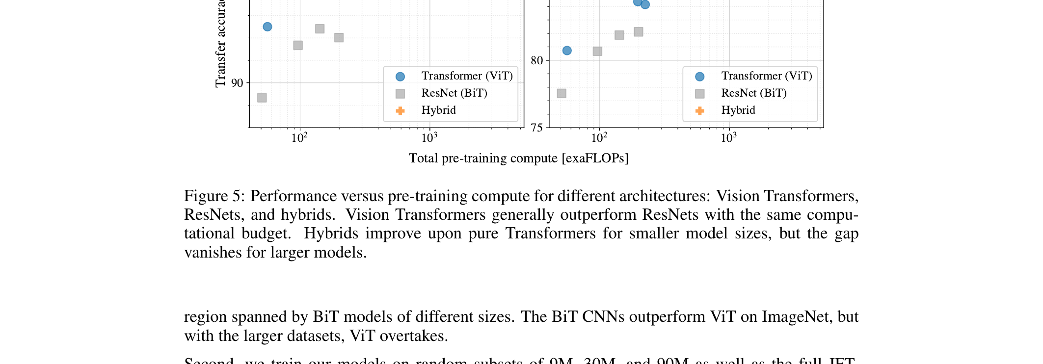
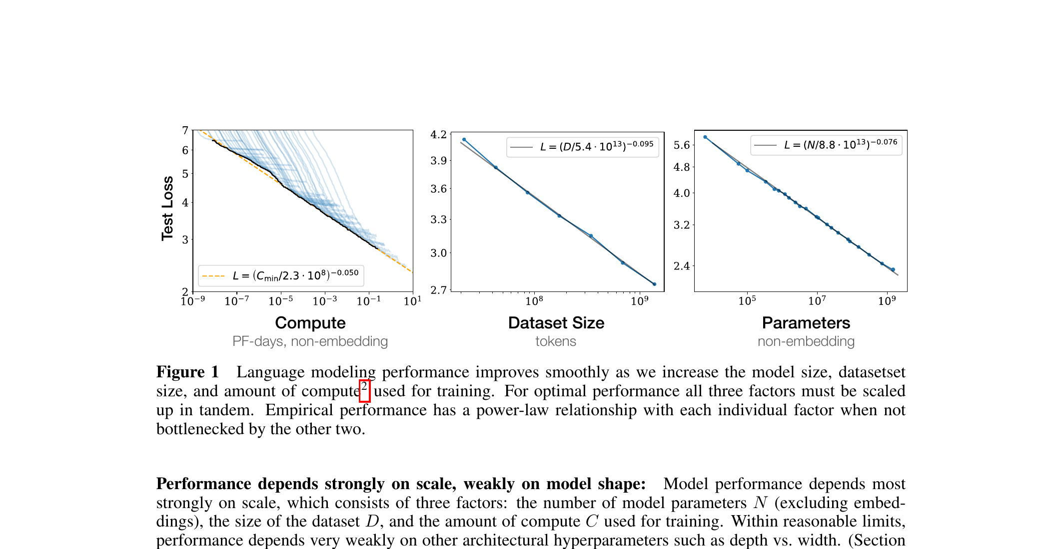
Why scaling won
- Transformers scale gracefully: doubling parameters and data gives predictable performance gains (scaling laws — Kaplan et al., Hoffmann et al.).
- Self-attention has no built-in inductive bias — which sounds bad — but means the model is flexible: with enough data, it learns the right priors.
- Hardware loves matmul; transformers are mostly matmul. GPUs and TPUs were designed around them (or vice versa).
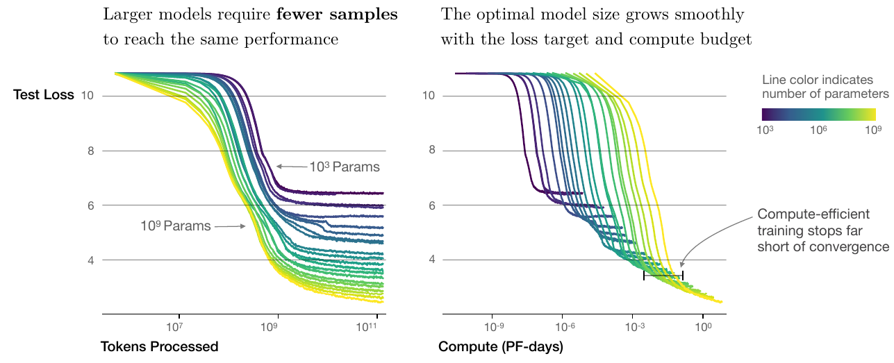
- Bigger is also more sample-efficient: a larger model reaches a target loss in fewer tokens — and compute-optimal training deliberately stops short of convergence (the seed of the Chinchilla allocation result).
- Result: the same architecture, scaled up with more data and compute, kept getting better.