Mathematical Foundations of AI & ML
Unit 11: Generative Models — VAE & Diffusion


What is a generative model?
A generative model represents (or approximates) the data distribution \(p(x)\). It must support:
- Sampling: produce \(x \sim p(x)\).
- Likelihood (sometimes): evaluate \(p(x)\) for a given \(x\).
- Conditioning: sample from \(p(x \mid c)\) for a condition \(c\) (target property, class label, prompt).
Today: VAEs (sampling + approximate likelihood) and diffusion (sampling, no exact likelihood, but extraordinary quality).
VAE — the architectural change
Vanilla AE:
\[ x \xrightarrow{f_\phi} z \xrightarrow{g_\theta} \hat x \]
Encoder produces a single point \(z\).
VAE:
\[ x \xrightarrow{f_\phi} (\mu, \sigma) \xrightarrow{\text{sample}} z \xrightarrow{g_\theta} \hat x \]
Encoder produces a distribution \(\mathcal{N}(\mu, \sigma^2 I)\). Sample \(z\) from it.
The latent \(z\) is now a random variable, not a deterministic function of \(x\).
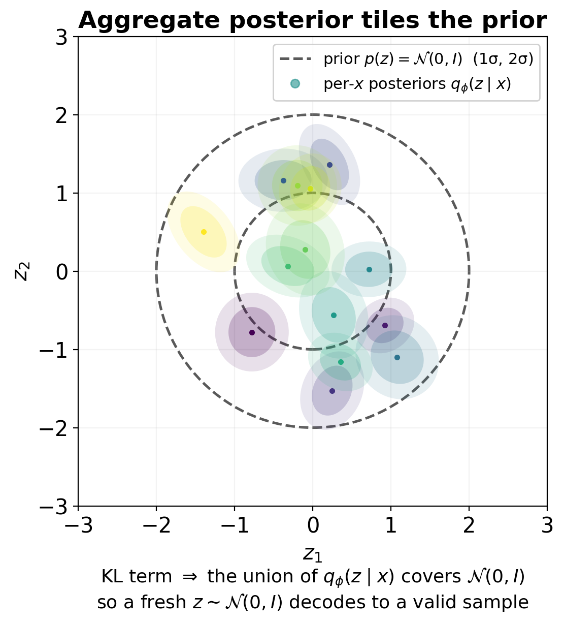
VAE — the prior on \(z\)
- We want a tractable distribution to sample from at generation time.
- Choose a fixed prior \(p(z) = \mathcal{N}(0, I)\) — the standard Gaussian on \(\mathbb{R}^k\).
- Constrain training so that the aggregate posterior \(q_\phi(z) = \mathbb{E}_{x}[q_\phi(z \mid x)]\) stays close to \(p(z)\).
- At generation time: sample \(z \sim \mathcal{N}(0, I)\), decode.
This is the core trick: train the encoder to push latents toward a known prior, so we can sample from that prior at test time.
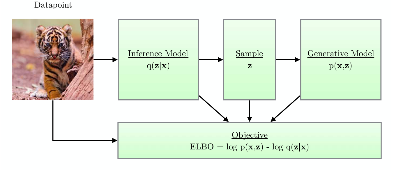
VAE — the loss, intuitively
For each training point \(x\), the VAE loss has two terms:
- Reconstruction term: how well does decoding \(z\) recover \(x\)? (Same as a vanilla AE.)
- Prior-matching term: is \(q_\phi(z \mid x)\) close to \(p(z) = \mathcal{N}(0, I)\)? Use KL divergence.
\[ \mathcal{L}(\theta, \phi; x) = \underbrace{-\mathbb{E}_{z \sim q_\phi(z|x)}[\log p_\theta(x \mid z)]}_{\text{reconstruction}} + \underbrace{\mathrm{KL}(q_\phi(z \mid x) \,\|\, p(z))}_{\text{prior-matching}} \]
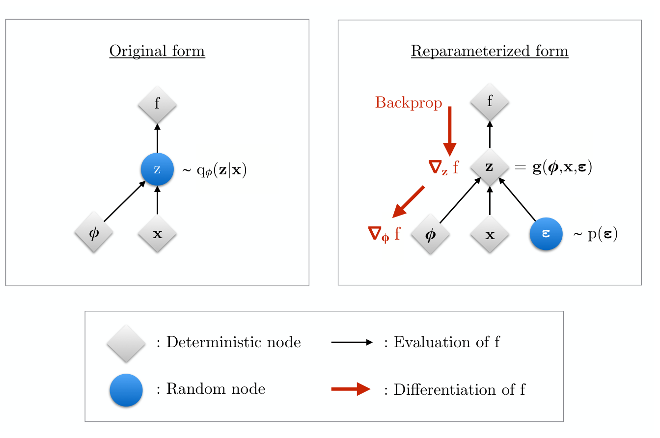
The reparameterization trick
- We need to backpropagate through the sampling step \(z \sim \mathcal{N}(\mu, \sigma^2)\).
- Problem: sampling is not differentiable — you cannot push \(\nabla_\phi\) through a random node.
- Fix: externalize the randomness. Rewrite the sample as a deterministic, differentiable function of a parameter-free noise variable: \[ z = \mu_\phi(x) + \sigma_\phi(x) \odot \epsilon, \quad \epsilon \sim \mathcal{N}(0, I). \]
Why it works: the gradient and the expectation now commute, giving a one-sample Monte-Carlo estimator: \[ \nabla_\phi\, \mathbb{E}_{q_\phi(z|x)}[f(z)] = \mathbb{E}_{p(\epsilon)}\!\big[\nabla_\phi f(z)\big] \approx \nabla_\phi f(z),\quad z=\mu_\phi+\sigma_\phi\odot\epsilon. \] The randomness sits in \(\epsilon\) (no parameters); the estimate is unbiased.
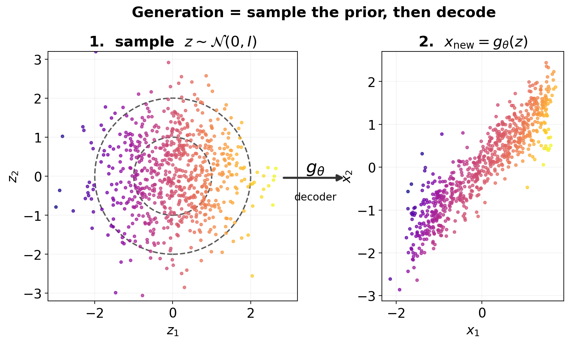
Generating new data from a trained VAE
- Sample \(z \sim \mathcal{N}(0, I)\).
- Decode: \(x_{\text{new}} = g_\theta(z)\).
- (Optional) for a stochastic decoder: also sample \(x \sim p_\theta(x \mid z)\).
That’s it. No labels needed; no special procedure. The trained encoder/decoder pair is now also a sampler.
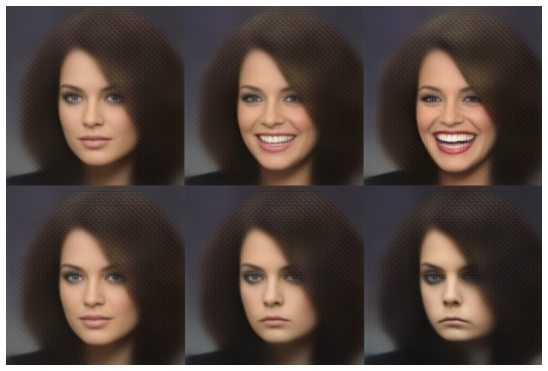
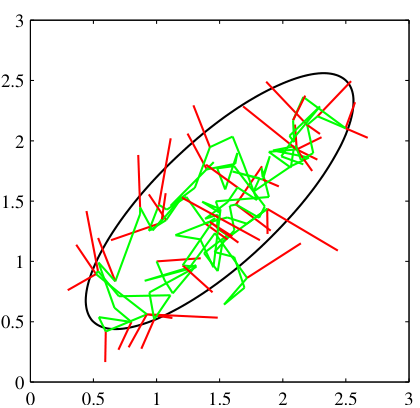
Latent interpolation in a VAE
- Encode two real samples \(x_A, x_B\) → latents \(z_A, z_B\).
- Interpolate: \(z_t = (1-t) z_A + t z_B\) for \(t \in [0, 1]\).
- Decode each \(z_t\).
- Result in a well-trained VAE: a smooth path between the two outputs in \(x\)-space.
- Same idea with an attribute direction: move \(z\) along a learned vector (e.g. a “smile vector”) to edit one factor at a time.
For materials: interpolate between two micrographs to see how phases transition; interpolate between two compositions to traverse phase space.
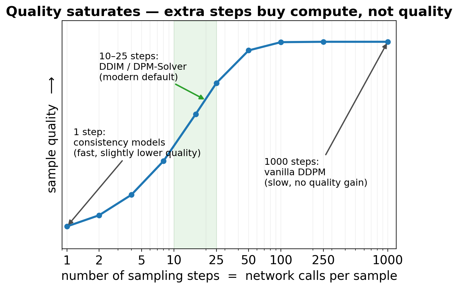
VAEs sample in one step. What if we used many?
- A VAE samples \(z\) from a learned prior, then decodes in one step.
- The single-step decode has to do all the work — and produces blurry outputs.
- What if we generated through many small steps, each easier than the last?
This is the diffusion idea: start from pure noise, gradually denoise to produce a sample.
Analogy: diffusion also iterates many small denoising steps. Unlike MCMC, the denoiser is a learned neural network.
The diffusion picture
- Forward process (fixed, no learning): gradually add Gaussian noise to data.
- Reverse process (learned): gradually remove noise to recover data.
- At training time: pick a random timestep \(t\), add the right amount of noise to a real sample, train a network to predict the noise.
- At generation time: start from \(x_T \sim \mathcal{N}(0, I)\), iterate the learned reverse process.
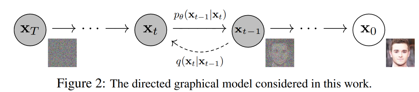
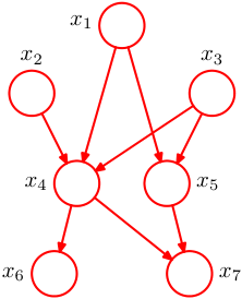
The directed graphical model of a diffusion model: the reverse process \(p_\theta(\mathbf{x}_{t-1}\mid\mathbf{x}_t)\) (solid arrows) gradually denoises from \(\mathbf{x}_T\) to \(\mathbf{x}_0\); the forward process \(q(\mathbf{x}_t\mid\mathbf{x}_{t-1})\) (dashed) adds noise. Source: (Ho et al. 2020) Fig. 2 (arXiv 2006.11239).
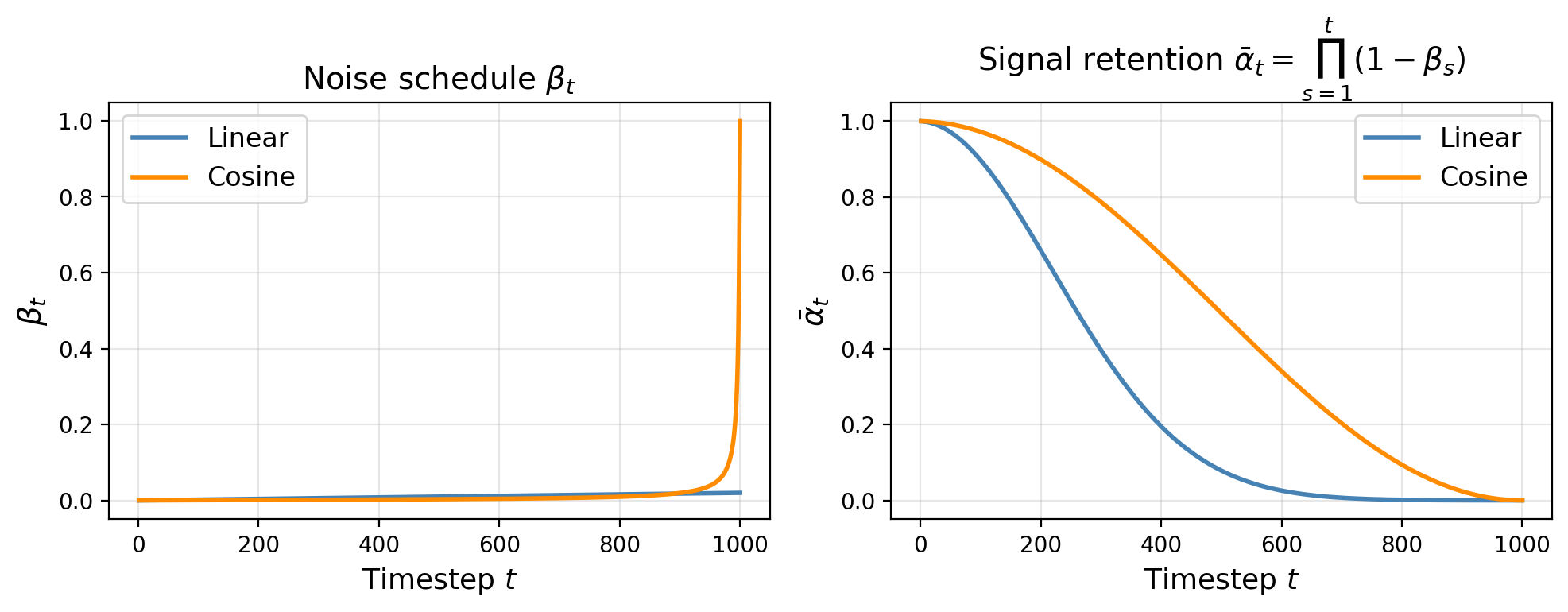
What the schedule looks like
- \(t = 0\): pure data. \(\bar\alpha_0 = 1\), no noise.
- \(t \approx T/2\): half noise, half data. The hard regime — both signal and noise visible.
- \(t = T\): \(\bar\alpha_T \approx 0\). Effectively pure Gaussian noise.
- Total steps \(T\): typically 1000 in DDPM, fewer (50–250) in modern accelerated samplers.
- Cosine schedule (Nichol and Dhariwal 2021): \(\bar\alpha_t = \cos^2\!\left(\tfrac{t/T+s}{1+s}\tfrac{\pi}{2}\right)/\cos^2\!\left(\tfrac{s}{1+s}\tfrac{\pi}{2}\right)\). Keeps signal longer at early steps; avoids abrupt destruction.
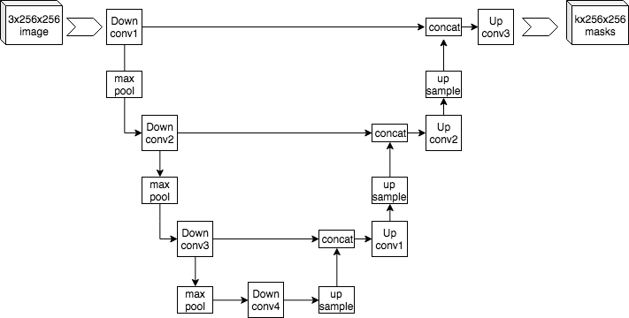
What is \(\epsilon_\theta\)?
- A neural network that takes a noisy image and a timestep, outputs predicted noise.
- Most common architecture: a U-Net (Ronneberger et al. 2015) with timestep embedding (sinusoidal).
- Contracting path encodes context; expansive path restores resolution with skip connections.
- Modern alternative: a transformer (DiT — Diffusion Transformer; Stable Diffusion 3).
- Receives time \(t\) as an additional input — same network handles all timesteps.
Sampling from a trained diffusion model
Input:  trained ε_θ
1. x_T ← sample from N(0, I)
2. for t = T, T-1, ..., 1:
3.     ε̂ ← ε_θ(x_t, t)
4.     compute mean μ_t and variance σ_t² from ε̂
5.     x_{t-1} ← μ_t + σ_t · z   (z=0 at t=1)
6. return x_0
\(T\) network calls per sample. With \(T = 1000\), this is slow compared to a VAE (1 call) — the dominant practical limitation.
What the sampling loop is really doing
- A trained denoiser doesn’t just clean an image — its correction points toward more realistic data.
- So each reverse step is just: take a small step in the denoiser’s direction, then add a little fresh noise.
- Picture a ball rolling downhill toward the data, with a bit of jitter to keep exploring — a random walk that drifts toward realistic samples.
- The jitter amount is a temperature knob: too low → samples collapse to one over-smoothed answer; too high → noise; balanced → realistic and diverse.
- DDPM, score models and NCSN are all the same “denoise a bit, add noise, repeat” recipe with different settings (Park et al. 2025).
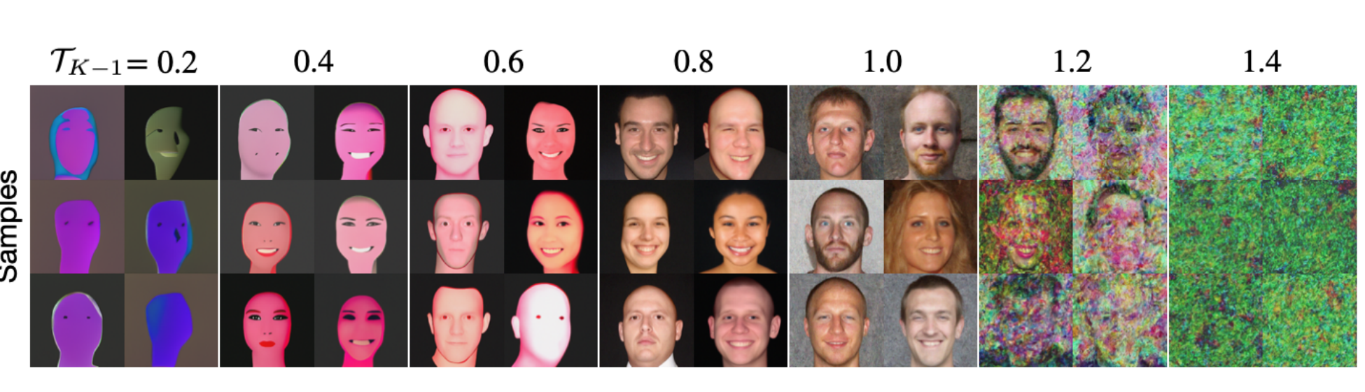
Same sampler, different ending temperature (jitter level). Too low → over-smoothed, low-variety faces; too high → noise; the balanced setting gives realistic, diverse samples. Source: (Park et al. 2025) Fig. 3.
Coarse structure first, fine detail last
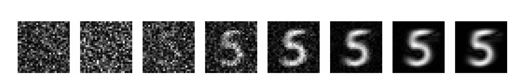
A digit forming from pure noise, reverse process left → right: structureless noise → a rough blob → the identity (“5”) → sharp detail. Large-scale structure emerges early, fine detail late. Source: (Weitzner et al. 2025) Fig. 1.
- Watch a sample form: the coarse, low-frequency structure appears first; the fine, high-frequency detail fills in last.
- Why: in the simplest (linear) case the optimal denoiser is exactly a PCA projection (Unit 2!). Early steps recover the top principal components — the largest-variance, coarsest structure; later steps add the smaller components — fine texture (Weitzner et al. 2025).
- This is why a half-finished diffusion sample already “looks like” the right object: the identity is set early, the polish comes late.
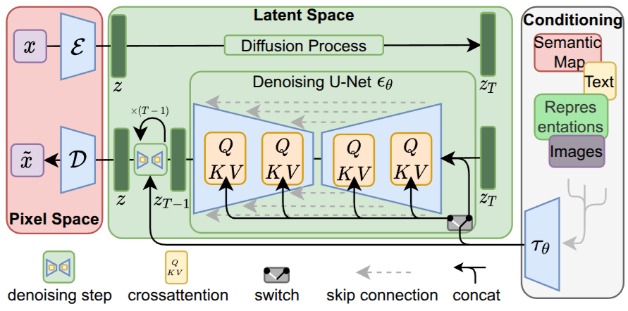
Latent diffusion (briefly)
- Diffusion in pixel space is expensive: 1024×1024 images mean huge networks.
- Latent diffusion (Rombach et al. 2022) (Stable Diffusion): train a VAE first, then run diffusion in the VAE’s latent space (e.g., 64×64 latents from 512×512 images).
- 64× fewer pixels in the diffusion process. Fast and high-quality.
- VAE + diffusion together — both halves of today’s lecture in one model.
- Conditioning (text, semantic map, class) via cross-attention inside the U-Net.