ECLIPSE Presentations – Mathematical Foundations of AI & ML Unit 12: Uncertainty in Predictions

Title + Unit 12 positioning

Unit 11 discovered structure in data. Unit 12 asks: how confident are our predictions?
Single-point predictions are insufficient for engineering decisions.
We need principled uncertainty quantification — from Bayesian inference to Gaussian Processes.

Open by naming the arc of the whole second half: Units 9–11 were about representation (latent spaces, attention, generative models) — squeezing structure out of data. This unit pivots from “what did the model learn” to “how much should we trust what it says.” That reframing is the entire point; say it before any math.
One-sentence stakes for a materials cohort: a regression model that says “yield strength = 450 MPa” is not a usable engineering object — a decision needs the bar around it. The number without the bar is the most dangerous artifact in applied ML.
Plant the destination: by minute 85 they will have a method (a GP) that honestly widens its error bars where it has no data, its scalable imitations (dropout, ensembles, MDN), and the calibration audit that checks whether any of those bars can be trusted. Tell them that payoff now so the Bayesian middle has a target.
Timing contract: ~10 min framing, ~15 min Bayesian predictive + variance split, ~15 min evidence, ~20 min GPs, ~15 min practical UQ, ~10 min calibration + materials. The checkpoints are your pace-recovery valves.

Learning outcomes for Unit 12

By the end of this lecture, students can:

derive the Bayesian predictive distribution and interpret the variance decomposition,
describe the evidence framework and the concept of effective parameters,
define a GP, derive its posterior, and interpret uncertainty bands,
compare practical UQ methods: MC Dropout, ensembles, and MDNs.

Don’t read the list — use it as a contract. Each bullet maps to one block of the lecture and to one of the “10 must-know statements” at the end; tell them that explicitly so they know the exam surface is fixed and visible.
Flag the two outcomes students underestimate: (1) the variance decomposition — it is the conceptual spine of the unit and the most likely short-derivation exam question; (2) the GP posterior in closed form — they will be asked to write those two boxed formulas from memory.
Calibrate rigor: we derive to the point of insight (the predictive integral, the GP conditioning result), not measure-theoretic completeness. This is a foundations-for-engineers course; the test is “can you put a defensible error bar on a prediction,” not “can you prove a theorem.”

Why point predictions are not enough

A model predicting 450 MPa tensile strength is useless without knowing if the uncertainty is $\pm 5$ or $\pm 100$ MPa.
In safety-critical applications, the uncertainty drives the decision, not the prediction.
Overconfident models are more dangerous than inaccurate ones.

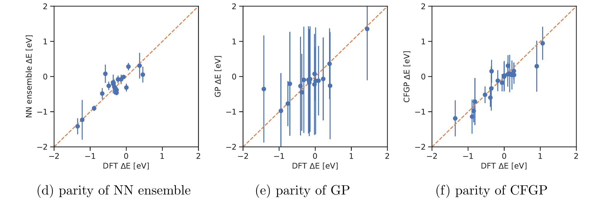
Same predictions, different error bars: an overconfident NN ensemble (left, bars too small — points miss the diagonal), an underconfident GP (middle, bars too large), and a well-calibrated model (right). The point estimates look similar; only the honesty of the error bar differs. Source: (Tran et al. 2020) Fig. 4 (parity plots, formation-energy $\Delta E$).

The figure is the payoff for the whole slide: three models with nearly identical point predictions (all cluster on the diagonal) but wildly different error bars — the NN ensemble’s bars are too small (overconfident: points fall outside their bars), the GP’s are too large (underconfident), the calibrated model’s are right. Say: “the mean is the same; the bar is where the trust lives — and a small bar is not the same as a correct one.” Materials-relevant (DFT formation-energy prediction), which pre-empts “this is just an image-classification problem.”
Tie to the three bullets: bullet 1 (±5 vs ±100) = the bar’s width; bullet 3 (overconfidence is dangerous) = the left panel literally — tiny bars that miss the truth are the failure mode you ship. Forward link: the GP (middle) is deliberately conservative; the next sections build toward calibrated bars.
Land the third bullet hard — it is the moral of the unit. An inaccurate-but-honest model says “I don’t know” and you go collect data; an overconfident model says “450 ± 3” when the truth is ±80 and you ship a part that fails. Wrong-and-loud beats wrong-and-quiet only for the person who isn’t liable.
Make the ±5 vs ±100 concrete: same point estimate, completely different engineering action — one passes a safety factor, the other forbids the design. The decision lives entirely in the bar, not the mean.
Misconception to preempt: students equate “good model” with “low test error.” Reframe — a model can have great average error and be catastrophically miscalibrated on the tail you actually care about. Average accuracy is necessary, not sufficient.
Transition: “So we need predictions that are distributions, not points. The cleanest way to get there is to stop committing to a single parameter value — that is the Bayesian predictive distribution.”

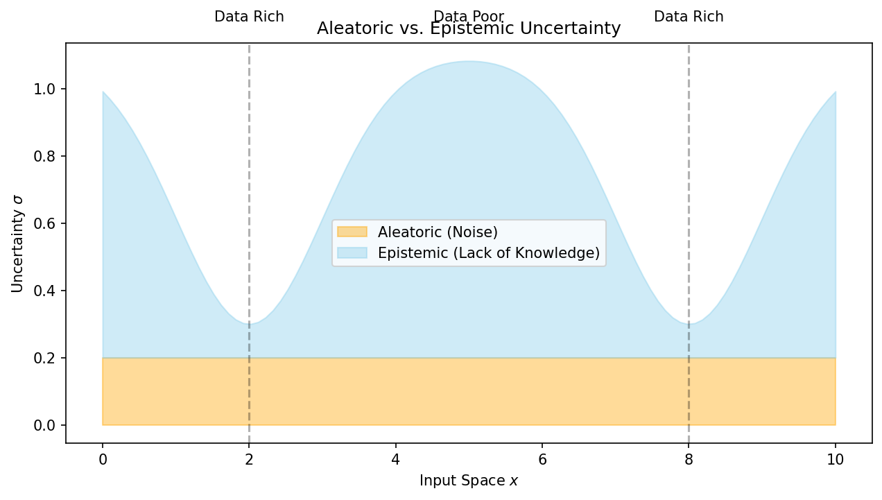
Recall: aleatory vs epistemic uncertainty (Unit 7)

Aleatory: inherent noise in the data-generating process — irreducible.
Epistemic: uncertainty from limited data or model capacity — reducible.
A complete UQ framework must quantify and distinguish both types.
As training data grows, epistemic uncertainty should shrink; aleatory uncertainty should not.

Aleatory (constant noise floor) vs epistemic (grows away from data) uncertainty decomposition.

This is a deliberate callback to Unit 7 — say “you have seen this,” then make it operational rather than philosophical. The new content is the shape in the figure: aleatory is a flat noise floor; epistemic balloons where there is no data. That picture is the visual the entire GP section pays off.
The examinable test of understanding: “you collect 10× more data — which band shrinks?” Only epistemic. Students who can’t answer this instantly are not ready for the variance decomposition two slides on; ask it aloud as a temperature check.
Materials anchor: aleatory = grain-to-grain scatter in a hardness measurement, irreducible at the modeling scale. Epistemic = you have tested only 3 compositions and are predicting a 4th — that shrinks the moment you synthesize it.
Forward link: “Keep this picture. In 20 minutes the GP will reproduce exactly this figure with no hand-tuning — narrow on data, wide off it. That is why GPs are the reference method for honest UQ.”

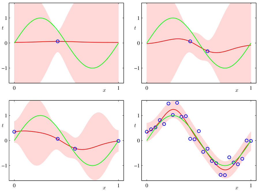
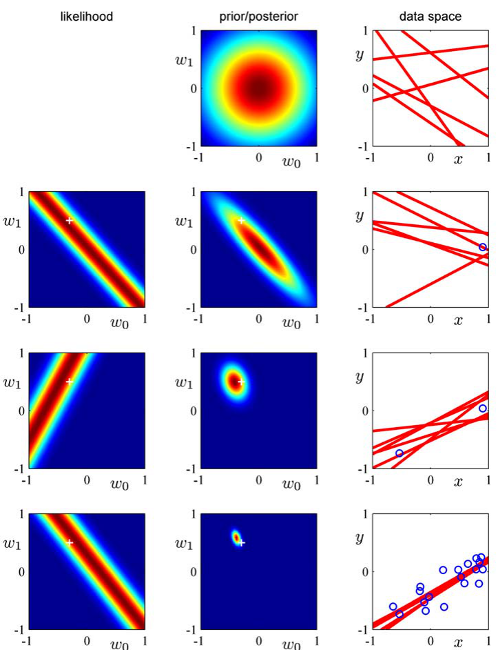
The Bayesian predictive distribution

Instead of predicting with a single $\hat{\theta}$, integrate over all plausible $\theta$:

\[ p(\mathbf{y}^* | \mathbf{x}^*, \mathcal{D}) = \int p(\mathbf{y}^* | \mathbf{x}^*, \theta) \, p(\theta | \mathcal{D}) \, d\theta \]

This accounts for parameter uncertainty — the full posterior contributes to the prediction.
The result is a distribution over predictions, not a single point.
As data increases (1 → 2 → 20 obs.), the predictive band narrows.

Bayesian predictive distribution: pink band = $\pm 2\sigma$ credible interval, narrows as training data grows. (Bishop 2006, fig. 3.8)

Read the integral aloud as an English sentence: “for every parameter the data finds plausible, ask what it predicts, then average those predictions weighted by how plausible the parameter is.” That sentence is the lecture; the symbols are bookkeeping.
Contrast with the plug-in estimate they know: MLE/MAP picks one $\hat\theta$ and is blind to the fact that nearby $\theta$ explain the data almost as well. The integral keeps that disagreement and propagates it into the prediction — that is where the error bar comes from.
Misconception to kill: this is not “averaging several models for accuracy” (ensembling) — it is the mathematically correct way to express not knowing $\theta$. The width is a feature, not noise to be smoothed away.
Tie to the figure: the band narrowing from 1→2→20 observations is the epistemic term from the previous slide collapsing. Same story, now with an equation. Transition: “How much of that width is reducible? Decompose it.”

Variance decomposition

\[ \text{Var}[\mathbf{y}^*] = \underbrace{\mathbb{E}_\theta[\sigma^2(\theta)]}_{\text{aleatory}} + \underbrace{\text{Var}_\theta[\boldsymbol{\mu}(\theta)]}_{\text{epistemic}} \]

Aleatory component: average noise variance across parameter values.

Epistemic component: how much the prediction mean varies across plausible parameters.

The epistemic term shrinks with more data; the aleatory term does not.

This is the conceptual keystone of the entire unit and the highest-probability derivation question on the exam. Spend real time. It is the law of total variance applied to predictions: “noise within each model” + “disagreement between models.”
Derive it in one line on the chalkboard if time allows: $\mathrm{Var}[y^*] = \mathbb{E}_\theta[\mathrm{Var}(y^*\mid\theta)] + \mathrm{Var}_\theta[\mathbb{E}(y^*\mid\theta)]$ — then name each piece. Students who see it fall out of total variance never forget it; students who memorize the boxed form forget it by the exam.
The single most important sentence in the unit: “More data attacks only the second term.” Say it, write it, and reuse the phrase verbatim at the GP slides and the active-learning slide so it becomes a refrain.
Misconception: that a flexible enough model can drive total variance to zero. No — the first term is the irreducible Bayes floor from Unit 7/8. Honesty means reporting it, not pretending it away.

Point estimates vs full distributions

Approach	Output	Uncertainty	Cost
MLE/MAP	Single $\hat{\mathbf{y}}$	None (or ad-hoc)	Low
Bayesian (exact)	Full $p(\mathbf{y}^\|\mathbf{x}^,\mathcal{D})$	Principled	High
Bayesian (approx.)	Approximate distribution	Approximate	Moderate

Use this table as the map for the rest of the lecture: every method we cover is one row. GPs are “Bayesian (exact)”; MC Dropout / VI are “Bayesian (approx.)”; ensembles and MDNs live just off this table as practical surrogates. Point at the row before each method block so students always know where they are.
The honest framing of the cost column: “principled” and “cheap” are in tension all unit. The engineering skill is not knowing the most rigorous method — it is choosing the cheapest row that still gives a defensible bar for the decision at hand.
Note the “(or ad-hoc)” on MLE: people do bolt error bars onto point estimates (bootstrap, a variance head). It can work, but it has no consistency guarantee — flag this so the calibration section later lands as “the audit that catches exactly this.”

When uncertainty matters most

Safety-critical: structural components, medical devices — failure consequences are severe.
Expensive experiments: each new alloy costs $10K to synthesize — guide experiments with uncertainty.
Extrapolation: new compositions, extreme conditions — the model is outside its training domain.
Active learning: acquire data where uncertainty is highest for maximum information gain.

This slide answers the student’s silent “why should I care” — make it concrete to their domain in every bullet, not abstract. The materials cohort lives in the second and third bullets daily: experiments are slow and expensive, and the interesting compositions are always extrapolative.
The extrapolation bullet is the one to dwell on: a model is most confident-sounding exactly where it is most wrong — far from training data a plug-in NN extrapolates a smooth line with no warning. A good UQ method must raise its hand there. This is the criterion we judge every method against.
The active-learning bullet is a forward hook to slides 44–45: “uncertainty isn’t only for reporting — it tells you which experiment to run next.” Plant it now, pay it off there.
Transition: “These needs are real. The rest of the lecture is a toolbox to meet them — here is the map.”

Practical UQ: a taxonomy

Exact Bayesian: Gaussian Processes — closed-form posterior, principled, but $O(N^3)$.
Approximate Bayesian: MC Dropout, variational inference — scale to large data, approximate.

Frequentist ensembles: deep ensembles — no Bayesian formalism, practical uncertainty from disagreement.
Direct prediction: MDNs — predict distribution parameters directly.

Roadmap of today’s 90 min

10–25 min: Bayesian predictive distribution and variance decomposition.
25–40 min: Evidence framework, marginal likelihood, effective parameters.
40–60 min: Gaussian Processes — definition, posterior, uncertainty bands.
60–75 min: Practical UQ — MC Dropout, ensembles, MDNs, stochastic enrichment.
75–85 min: Calibration and engineering applications.

The marginal likelihood (evidence)

\[ p(\mathcal{D} | \mathcal{M}) = \int p(\mathcal{D} | \theta, \mathcal{M}) \, p(\theta | \mathcal{M}) \, d\theta \]

Measures how well model $\mathcal{M}$ explains the data, averaging over all parameter values.
Automatically balances fit (likelihood) and complexity (prior spread) (Murphy 2012).

Frame the structural parallel explicitly: this is the same integral as the predictive distribution, but integrating the likelihood of the data instead of a new prediction. One machine — marginalize over $\theta$ — answers both “what do I predict” and “which model is best.” Students who see that unity stop treating these as separate topics.
The non-obvious idea worth slowing down on: a model that can fit anything spreads its prior probability thin over a huge data space, so it assigns low probability to the particular dataset you saw. Flexibility is paid for in the evidence. This is Occam’s razor falling out of probability with no penalty term bolted on.
Examinable phrase to dictate: “the evidence is the probability the model assigned to the data before seeing it, averaged over the prior.” Get them to write that sentence; it is the whole next three slides.

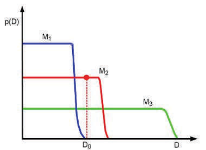
Evidence as automatic Occam’s razor

Simple model $\mathcal{M}_1$: prior concentrated on few parameter values → high evidence if data is simple.
Complex model $\mathcal{M}_3$: prior spread thinly over many parameters → lower evidence unless data demands complexity.
Just-right model $\mathcal{M}_2$: highest evidence at observed $\mathcal{D}_0$.
The evidence automatically penalizes unnecessary complexity — no need for explicit regularization.

Bayesian Occam’s razor: $M_2$ (red) has the highest evidence at the observed data $D_0$. (Murphy 2012, fig. 5.6)

Drive the figure, not the bullets. Every distribution integrates to one along the data axis — so a model that “could explain many datasets” must be flatter and lower on the one you actually observed. That conservation-of-probability argument is the entire intuition; draw it with your hand on the screen.
The punchline that surprises students: there is no $\lambda$, no penalty term, no held-out set. Complexity control is a consequence of normalization, not an ingredient you add. Contrast with the explicit regularizer from Unit 8 — same effect, derived rather than imposed.
Honesty caveat to state: this is exact only if you can compute the integral, which you usually can’t for deep nets — that is why we still cross-validate in practice. The evidence is the principle; the GP marginal likelihood later is the rare case where it is computable in closed form.

Model comparison via evidence

Bayes factor: $\frac{p(\mathcal{M}_1 | \mathcal{D})}{p(\mathcal{M}_2 | \mathcal{D})} = \frac{p(\mathcal{D} | \mathcal{M}_1)}{p(\mathcal{D} | \mathcal{M}_2)} \cdot \frac{p(\mathcal{M}_1)}{p(\mathcal{M}_2)}$.
With equal model priors: the model with higher evidence is preferred.
Unlike cross-validation, this uses all the data for both fitting and evaluation.
Evidence selects $d{=}1$ (linear) over $d{=}2,3$ for small $N{=}5$; at $N{=}30$ it correctly selects $d{=}2$.

Polynomial regression ($d{=}1,2,3$) on $N{=}5$ points: dotted bands show $\pm\sigma$ predictive uncertainty. Bottom-right: posterior $p(M|D)$ — degree 1 wins at small $N$. (Murphy 2012, fig. 5.7)

The data-efficiency point is the one to sell: cross-validation throws away a fold to estimate generalization; the evidence uses every point for both fitting and model scoring because it never needs a held-out set — the prior-averaging is the regularization. For a 50-sample alloy dataset that difference is decisive.
Make the last bullet a story about adaptivity: with 5 points, “degree 1” is not the true model — it is the appropriately humble model. As data arrives the evidence promotes degree 2. The right complexity is a function of how much you know, and the evidence tracks that automatically.
Caution to state plainly: Bayes factors are notoriously sensitive to the prior (unlike the posterior, which washes the prior out with data). Mention it so they don’t over-trust a single number — and so empirical Bayes two slides on is motivated as “then choose the prior by the data too.”

Effective number of parameters

\[ \gamma = \sum_i \frac{\lambda_i}{\lambda_i + \alpha} \]

$\lambda_i$: eigenvalues of the data precision matrix. $\alpha$: prior precision.
$\gamma \leq$ total number of parameters. Often $\gamma \ll$ total parameters.
Interpretation: only $\gamma$ parameters are effectively constrained by the data (Bishop 2006).

Read each term in the sum as a soft switch in $[0,1]$: a direction the data constrains strongly ($\lambda_i \gg \alpha$) contributes ≈1 — “one real parameter”; a direction the data barely touches ($\lambda_i \ll \alpha$) contributes ≈0 — “the prior is holding this one up, not the data.” $\gamma$ just counts how many parameters the data is actually paying for.
This dissolves a paradox students carry: a model can have a million weights and still not overfit if the data only pins down a few hundred effective directions. Parameter count is the wrong complexity measure; $\gamma$ is the right one. Forward link: this is the seed of the double-descent / over-parameterization story they’ll meet later.
Keep it conceptual — the eigen-decomposition derivation is exercise/optional-depth (Bishop 3.5). The examinable claim is the interpretation sentence, not the spectral algebra.

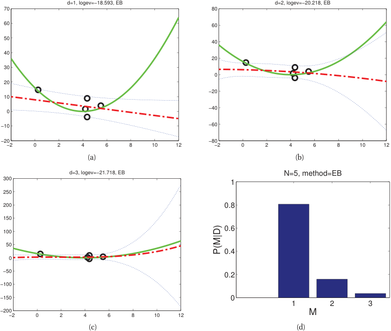
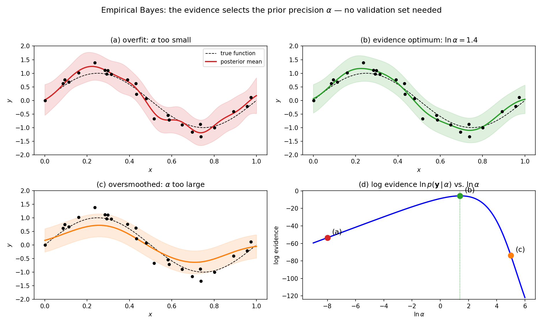
Empirical Bayes

Instead of fixing hyperparameters (prior variance, noise level), optimize them by maximizing the evidence.
$\hat{\alpha}, \hat{\sigma}^2 = \arg\max_{\alpha, \sigma^2} \log p(\mathcal{D} | \alpha, \sigma^2)$.
This is a principled alternative to cross-validation for hyperparameter selection.
Also called type-II maximum likelihood.
Example →: RBF-basis regression, prior $\mathbf{w} \sim \mathcal{N}(\mathbf{0}, \alpha^{-1}\mathbf{I})$. The evidence curve (d) picks the $\alpha$ of fit (b) — using all the data, no validation set.

Name the level shift clearly: ordinary MLE fits parameters; empirical Bayes does MLE one floor up — it fits the hyperparameters by maximizing the evidence, with $\theta$ already integrated out. “Type-II ML” is just that one-sentence idea; the jargon hides how simple it is.
Walk the figure as a story, panel by panel: (a) tiny $\alpha$ = broad prior = the model buys every wiggle the noise sells; (c) huge $\alpha$ = prior strangles the weights = the fit collapses toward zero; (b) the evidence’s choice, found by sliding along curve (d) to its peak. The punchline: nobody held out data — panel (d) is computed from the same 25 points being fit. The Occam argument from three slides ago is what makes that legal: the evidence already charges for complexity.
Note $\alpha$ is the same $\alpha$ as in the effective-parameters formula $\gamma = \sum_i \lambda_i/(\lambda_i + \alpha)$ two slides back — the knob the evidence is turning is exactly the one that decides how many parameters the data is allowed to pay for. Two slides, one machine.
This is the slide that makes GPs practical, so flag the forward link hard: “Remember this — in 20 minutes ‘learn the GP length scale by maximizing the marginal likelihood’ is literally this slide, with $\alpha$ swapped for $(\ell, \sigma_f, \sigma_n)$. The evidence section is not abstract; it is the GP’s training algorithm.”
Honest caveat: empirical Bayes can over-fit the hyperparameters when data is scarce (you used the data to pick the prior). Usually mild, occasionally not — worth one sentence so they don’t treat it as free.

Checkpoint: evidence interpretation

Question: Model A has 100 parameters and log-evidence −500. Model B has 10 parameters and log-evidence −480. Which is preferred?
Answer: Model B — higher evidence means it explains the data better relative to its complexity.

What is a Gaussian Process?

A GP is a distribution over functions: $f \sim \mathcal{GP}(m(\mathbf{x}), k(\mathbf{x}, \mathbf{x}'))$.
Any finite collection of function values $[f(\mathbf{x}_1), \dots, f(\mathbf{x}_N)]$ is jointly Gaussian.
The GP is fully specified by its mean function $m(\mathbf{x})$ and kernel function $k(\mathbf{x}, \mathbf{x}')$.

The conceptual leap, stated slowly: a Gaussian distribution is over vectors; a GP is over functions. The trick that makes that tractable is the second bullet — you never manipulate the infinite object, only its finite restriction at the inputs you care about, and that restriction is an ordinary multivariate Gaussian. Everything else is conditioning that Gaussian.
Walk the mermaid arrows aloud as the lecture roadmap for the next eight slides: prior (mean + kernel) → condition on data → posterior → read off uncertainty bands. Tell them every GP slide is one box in this chain so they can place each piece.
Anchor “distribution over functions” with the figure they will see at the prior slide: each draw is a whole curve, not a point. Promise it now: “in three slides you will see five random functions sampled from this thing — that is what the prior literally is.”

GP as infinite-dimensional Gaussian

A multivariate Gaussian is a distribution over vectors.
A GP extends this to a distribution over functions (infinite-dimensional objects).
The kernel function $k(\mathbf{x}, \mathbf{x}')$ plays the role of the covariance matrix.
This is a Bayesian nonparametric model — complexity grows with data (Murphy 2012).

The sentence that makes it click: “index the Gaussian by a continuous input instead of an integer.” A 3-vector Gaussian has a 3×3 covariance matrix; a GP has a covariance function $k(\mathbf{x},\mathbf{x}')$ that returns the entry for any pair of inputs, including ones you haven’t picked yet. Same object, continuous index.
Define “nonparametric” honestly so it isn’t a buzzword: not no parameters — the effective capacity grows with the data because the model keeps all training points around. Contrast with a fixed-width NN whose capacity is frozen at design time. This is also the seed of the $O(N^3)$ cost later — flag that the same property that makes it flexible makes it expensive.
Keep this slide short; it is the bridge between “what is a GP” and “so we must choose $m$ and $k$” — the next three slides.

From weight space to function space

Any linear-in-parameters model with a Gaussian prior on the weights is a GP:

\[ f(\mathbf{x}) = \mathbf{w}^\top \boldsymbol{\phi}(\mathbf{x}), \quad \mathbf{w} \sim \mathcal{N}(\mathbf{u}, \mathbf{S}) \;\Rightarrow\; f \sim \mathcal{GP}(m, k) \]

\[ m(\mathbf{x}) = \mathbf{u}^\top \boldsymbol{\phi}(\mathbf{x}), \qquad k(\mathbf{x}, \mathbf{x}') = \boldsymbol{\phi}(\mathbf{x})^\top \mathbf{S} \, \boldsymbol{\phi}(\mathbf{x}') \]

Example: $f(x) = w_0 + w_1 x$ with $w_0, w_1 \sim \mathcal{N}(0,1)$ gives $m(x) = 0$, $k(x,x') = 1 + xx'$.
Bayesian linear regression (Unit’s prerequisite!) is a GP with the linear kernel.

Sequential Bayesian learning of $f(x) = w_0 + w_1 x$: weight-space posterior (left) and the corresponding sampled functions (right) as observations arrive. (Bishop 2006, fig. 3.7)

This slide earns the GP its place in a foundations course: it is not a new exotic model but the function-space view of the Bayesian linear regression they already know. Derive the linear example live in two lines — $m(x) = \mathbb{E}[w_0 + w_1 x] = 0$; $k(x,x') = \mathbb{E}[(w_0 + w_1 x)(w_0 + w_1 x')] = 1 + xx'$ — it is thirty seconds of algebra and it demystifies the whole kernel concept: a kernel is what a prior over weights looks like from function space.
Now the Bishop figure is in its rightful home: the left column is the posterior contracting in weight space, the right column is the same contraction seen in function space. Same information, two coordinate systems. The GP’s proposition is that the right column is the one you can reason about — “smooth, slowly varying, periodic” are statements about functions, not about $w_{17}$.
The punchline to say explicitly: since $\boldsymbol{\phi}$ can be any basis — polynomials, Fourier modes, radial bumps — this construction covers a huge model class. The next slide pushes it to infinitely many basis functions and gets the RBF kernel.

The RBF kernel: infinitely many basis functions

Place $J$ Gaussian bumps $\phi_i(x) = \exp\left(-\frac{(x - c_i)^2}{2\ell^2}\right)$ at centers $c_i$, with $w_i \sim \mathcal{N}\!\left(0, \frac{\sigma^2}{J}\right)$:

\[ k(x, x') = \frac{\sigma^2}{J} \sum_{i=1}^{J} \phi_i(x)\,\phi_i(x') \]

Let $J \to \infty$ with centers spread over the whole real line — the sum becomes an integral:

\[ k(x,x') = \int_{-\infty}^{\infty} \phi_c(x)\,\phi_c(x')\, dc \;\propto\; \exp\!\left(-\frac{(x-x')^2}{2(\sqrt{2}\ell)^2}\right) \]

The RBF kernel is a model with infinitely many basis functions — evaluated with finite computation.
A GP with an RBF kernel is a universal approximator, yet does not overfit: complexity is controlled by the marginal likelihood, not the parameter count.

This is the “infinite parameters, finite compute” claim from two slides ago, now derived instead of asserted — the kernel trick in its cleanest form. Walk the limit slowly: each basis function is a bump of width $\ell$; as $J\to\infty$ the weighted sum becomes a Riemann integral; the Gaussian-times-Gaussian integral evaluates in closed form to… a Gaussian in $(x - x')$. The RBF kernel is the covariance of infinitely many radial bumps.
Connect to the effective-parameters slide: infinitely many nominal parameters, yet $\gamma$ — the number the data actually pays for — stays finite and modest. That is why an RBF-GP does not overfit despite infinite capacity: the evidence machinery from the first half of the lecture is doing the complexity control automatically. Two blocks of the lecture just clicked together; point at it.
One-sentence bridge for the deep-learning students: the same construction applied to a one-hidden-layer network with infinitely many units (via CLT) gives the neural network kernel — infinitely wide NNs are GPs. Mention by name only; it reframes the NN-vs-GP debate as “not as distinct as they look” and seeds the deep-kernel-learning pointer in the DSEM course.

Mean function m(x)

$m(\mathbf{x}) = \mathbb{E}[f(\mathbf{x})]$: the expected function value at each input.
Common choice: $m(\mathbf{x}) = 0$ (zero-mean prior).
Can encode prior knowledge: $m(\mathbf{x}) = a\mathbf{x} + b$ for a linear trend.
The mean function is updated to the posterior mean after observing data.

Preempt the obvious worry: “zero mean? all my yield strengths are ≈400 MPa.” Reassure — zero-mean is a statement about the prior away from data, and it is conventional to center/standardize targets first. Near data the posterior mean is driven entirely by the kernel and the observations, not by $m$.
The one place a non-zero mean earns its keep: known physics or a known trend. If theory says the property grows linearly with temperature, put that in $m(\mathbf{x})$ and let the GP model only the residual. Forward hook to Unit 13 (physics-informed): “an informative mean function is the simplest way to inject domain knowledge — we revisit this next unit.”
This is the lowest-leverage of the three GP-specification slides; spend the time budget on the kernel, where the modeling decisions actually live.

Kernel (covariance) function k(x, x’)

$k(\mathbf{x}, \mathbf{x}') = \text{Cov}[f(\mathbf{x}), f(\mathbf{x}')]$: encodes the correlation between function values.
The kernel determines the properties of sampled functions:
- Smoothness, periodicity, length scale, amplitude.
The kernel must be positive semi-definite (valid covariance matrix for any finite set of points).

This is the heart of GP modeling — say so. Choosing a kernel is choosing your prior beliefs about the function: “nearby inputs give similar outputs” is the entire content of the RBF kernel, and that one assumption is what produces the honest uncertainty bands later. The kernel is where the science goes in.
Build the core intuition in one sentence: $k$ large ⇒ the two function values are tied together ⇒ knowing one tells you a lot about the other; $k\to 0$ ⇒ they are independent ⇒ data here says nothing there. That is exactly why GP uncertainty grows away from data — the kernel decorrelates you from your observations. Plant this; it is the payoff at the uncertainty-band slide.
The PSD requirement: state it as the rule, not the proof — it just means “for any set of inputs the resulting matrix must be a legal covariance matrix (no negative variances).” Why some functions are invalid kernels is exercise/optional depth.

The RBF (squared exponential) kernel

\[ k(\mathbf{x}, \mathbf{x}') = \sigma_f^2 \exp\!\left(-\frac{\|\mathbf{x} - \mathbf{x}'\|^2}{2\ell^2}\right) \]

Length scale $\ell$: controls how far apart inputs can be and still be correlated.
Signal variance $\sigma_f^2$: controls the amplitude of function variation.
Produces infinitely differentiable (very smooth) functions.

Read the formula physically: correlation is 1 when $\mathbf{x}=\mathbf{x}'$ and decays smoothly to 0 as they separate, with $\ell$ setting “how far is far.” Beyond a few $\ell$ apart, two points are effectively independent — that distance is where the uncertainty band will balloon back to $\sigma_f$. Connect the two parameters to the two visible features of any GP plot now so the length-scale slide is a callback.
$\ell$ is the single most consequential knob in the unit and the most common exam target; $\sigma_f^2$ just rescales the vertical axis. Say which one to obsess over.
Honest caveat: “infinitely differentiable” is mathematically elegant and often too smooth for real signals with kinks — which is the entire motivation for the Matérn kernel on the next slide. Set up that contrast deliberately rather than presenting RBF as default-and-done.

Other kernels

Matérn: $k(\mathbf{x},\mathbf{x}') \propto$ Bessel function — adjustable smoothness via parameter $\nu$.
Periodic: captures repeating patterns.
Linear: $k(\mathbf{x},\mathbf{x}') = \sigma^2 \mathbf{x}^\top \mathbf{x}'$ — equivalent to Bayesian linear regression.
Composite: sums and products of kernels combine properties (e.g., smooth + periodic).

Don’t catalogue — teach the meta-point: the kernel is a modeling language, and each entry here is a vocabulary word for a belief about the function. Matérn = “smooth but not infinitely so” (the realistic default for physical signals). Periodic = “I know there’s a cycle.” Linear-kernel GP = Bayesian linear regression, a unification worth one sentence: GPs contain the models they already know.
The composite bullet has the leverage and the best demo line: “smooth long-term trend + seasonal cycle = RBF + Periodic” is the textbook Mauna Loa CO₂ model — literally the dataset in the MC Dropout figure later. Forward-link it so the course feels stitched together.
This whole slide is the first thing to cut if you hit 60 minutes behind — decide now which Matérn-vs-RBF sentence survives the cut (the “real signals aren’t infinitely smooth” one).

GP prior: sampling functions

Before seeing data, sample functions from the prior: $f \sim \mathcal{GP}(0, k)$.
With RBF kernel: smooth, random functions with length scale $\ell$ and amplitude $\sigma_f$.
Different kernel parameters produce visually different function families.
The prior encodes our beliefs about what functions are plausible.

Five sample functions drawn from a zero-mean GP prior with RBF kernel — each curve is one complete draw from the distribution over functions.

This is the slide that makes “distribution over functions” finally tangible — slow down and let them look. Each curve is one sample — one entire function drawn from the prior. The spread of the curves at a fixed $x$ is the prior uncertainty there. Trace one curve with your hand so they see it as a single draw, not a band.
Ask the room the modeling question the figure poses: “do these look like plausible candidates for your signal?” That is what choosing a prior means — you are not fitting anything yet, you are declaring which function families are on the table (how wiggly, what amplitude). If their physical signal is smoother or rougher than these draws, the kernel hyperparameters are wrong before any data arrives.
This is also the spine the next slide (posterior) hangs on — tell them “conditioning will take exactly this bundle of curves and force it through the observations; the next slide shows that happen.”

GP posterior: conditioning on data

Observe $\mathcal{D} = \{(\mathbf{x}_i, y_i)\}_{i=1}^N$ with $y_i = f(\mathbf{x}_i) + \epsilon$, $\epsilon \sim \mathcal{N}(0, \sigma_n^2)$.
The posterior $f | \mathcal{D}$ is also a GP with updated mean and covariance.
The posterior passes through (or near) the training points.
Away from data, the posterior reverts to the prior.

Sample functions from the GP *posterior*: the prior bundle from the previous slide, now forced through the observations — samples agree at the data and fan out in the gaps.

The figure is the direct sequel to the previous slide — same kind of sample curves, but now every one of them passes (near) the observations. Conditioning didn’t replace the prior; it filtered it. Say it that way: “these are the survivors of the prior.”
The structurally beautiful fact to emphasize: conditioning a GP on data gives another GP. The family is closed under observation — that is exactly why everything stays in closed form and why GPs are the “exact Bayesian” row of the taxonomy. No approximation enters here.
“Passes through (or near)”: the near is doing real work — it is the $\sigma_n^2$ noise term. With noisy observations the posterior mean should not interpolate every point exactly; forcing it through noisy data is overfitting. Tie $\sigma_n^2$ to the aleatory floor from the variance decomposition — same quantity, reappearing.
“Reverts to the prior away from data” is the one-sentence summary of honest uncertainty and a verbatim callback to the recall figure. Pause on it, then transition: “Now the formulas that produce exactly this picture — and you will be asked to write them.”

GP posterior: closed-form formulas

\[ \boldsymbol{\mu}^*(\mathbf{x}^*) = \mathbf{k}_*^\top (\mathbf{K} + \sigma_n^2 \mathbf{I})^{-1} \mathbf{y} \]

\[ \sigma^{*2}(\mathbf{x}^*) = k(\mathbf{x}^*, \mathbf{x}^*) - \mathbf{k}_*^\top (\mathbf{K} + \sigma_n^2 \mathbf{I})^{-1} \mathbf{k}_* \]

$\mathbf{K}$: kernel matrix $[k(\mathbf{x}_i, \mathbf{x}_j)]_{N \times N}$. $\mathbf{k}_*$: vector $[k(\mathbf{x}^*, \mathbf{x}_i)]$.
The key operation is inverting $(\mathbf{K} + \sigma_n^2 \mathbf{I})$ — cost $O(N^3)$.

These two boxes are the highest-yield memorization target in the unit — students will be asked to reproduce them. Reveal them one fragment at a time and narrate the structure rather than the symbols, because the structure is what’s memorable.
Mean, in words: “a weighted average of the training outputs $\mathbf{y}$, where the weights are how kernel-similar the query is to each training point.” A test point near training data leans on it; far away, $\mathbf{k}_*\to 0$ and the mean returns to the prior mean (0). Show them the limit on the board.
Variance, in words: “prior variance at the query minus what the data explains away.” The subtracted term is non-negative — observing data can only reduce variance, never increase it, and crucially the reduction does not depend on $\mathbf{y}$, only on where you sampled. That last fact is the entire theoretical basis for active learning (slide 45) — flag it now.
The $O(N^3)$ note is the seed of the cost slide; mention it lives in the matrix inverse so the limitation later is not a surprise.

GP posterior: interpretation

Mean $\boldsymbol{\mu}^*(\mathbf{x}^*)$: best prediction — a weighted combination of training outputs.
Variance $\sigma^{*2}(\mathbf{x}^*)$:
- Small near training data (low epistemic uncertainty).
- Large far from training data (high epistemic uncertainty).
- Approaches prior variance $\sigma_f^2$ as distance from data grows.

This slide is the plain-English decompression of the previous one — if the formulas felt abstract, this is where the room re-boards. Keep returning to “the variance only depends on where you have data, not on what the values were.” Students consistently find this surprising and it is genuinely deep: a GP knows it is uncertain in a gap before it has seen a single label there.
Connect the third sub-bullet straight back to the recall figure and the variance decomposition: “GP variance → $\sigma_f^2$ far from data” is literally the epistemic term not having been reduced. Same concept, third appearance — the repetition is intentional, name it as a refrain.
One-line exam framing: the GP gives you the variance decomposition for free and spatially resolved — $\sigma_n^2$ is the aleatory floor everywhere, the subtracted term is the locally-reducible epistemic part.

GP uncertainty bands

Plot $\boldsymbol{\mu}(\mathbf{x}) \pm 2\sigma(\mathbf{x})$: the 95% credible band.
Bands are narrow near observed data (confident predictions).
Bands widen away from data (uncertain predictions).
This is honest uncertainty — the GP admits what it does not know.

Posterior mean with 95% credible band — the sample-function bundle from the previous slide summarized as mean ± 2σ. The band collapses at observed points and expands in unsampled regions.

This is the emotional payoff of the entire GP block — let it land. Point at the figure: “This is the picture I promised you at the recall slide.” The band you drew by hand as ‘what good UQ should look like’ is now produced automatically by the posterior-variance formula, with no tuning of the shape. Make the closing of that loop explicit.
The word “honest” is the one to dwell on and contrast: a plug-in neural net draws a confident line straight through the data gap; the GP fans out and says “I don’t know here.” For a materials engineer deciding whether to trust an extrapolated composition, that fan-out is the most valuable output the model produces — more than the mean.
Numeric caveat worth one sentence: ±2σ ≈ 95% holds because the posterior is Gaussian. When we leave GPs for NNs (next block) that clean mapping breaks — which is precisely why we will need calibration. Plant the motivation here.

GP hyperparameter learning

Optimize kernel hyperparameters $\ell, \sigma_f, \sigma_n$ by maximizing the log marginal likelihood:

\[ \log p(\mathbf{y} | \mathbf{X}) = -\frac{1}{2}\mathbf{y}^\top(\mathbf{K} + \sigma_n^2 \mathbf{I})^{-1}\mathbf{y} - \frac{1}{2}\log|\mathbf{K} + \sigma_n^2 \mathbf{I}| - \frac{N}{2}\log 2\pi \]

Three terms: data fit, complexity penalty, normalization.
Gradient-based optimization (L-BFGS is common).

Log marginal likelihood surface (a) and the two GP fits at local optima: wiggly short-$\ell$ fit (b) vs smooth long-$\ell$ fit (c). (Murphy 2012, fig. 15.5)

Cash the promissory note from the empirical-Bayes slide: “I told you the evidence section was the GP’s training algorithm — here it is.” Walk the three terms and name the Occam tension explicitly: first term rewards fitting $\mathbf{y}$, second term ($\log|\mathbf{K}+\sigma_n^2 I|$) penalizes an over-flexible (short-$\ell$) kernel, third is a constant. The kernel is chosen by the same automatic-razor argument from the Occam slide — same machine, now differentiable.
The figure carries a sober warning: the marginal-likelihood surface is multimodal. The wiggly short-$\ell$ fit and the smooth long-$\ell$ fit are both local optima — different random restarts give different GPs. Say plainly: GP training is not the convex free lunch it’s sometimes sold as; restart and sanity-check the length scale against domain knowledge.
Examinable contrast to state: this replaces cross-validation for hyperparameters — one differentiable objective, all the data, no folds. That data efficiency is the practical reason GPs win on small materials datasets.

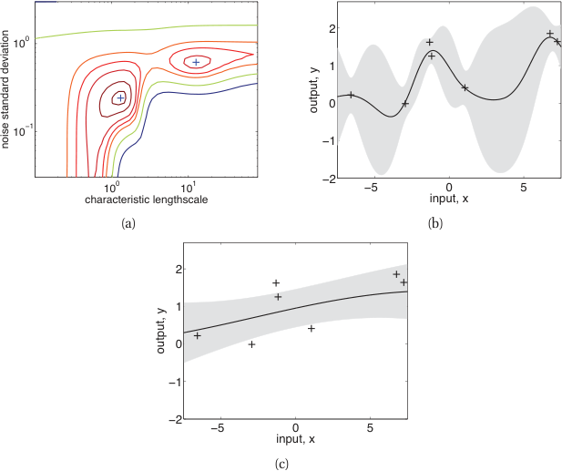
Length scale effect

Short $\ell$: wiggly functions, fits local patterns (and possibly noise).
Long $\ell$: smooth functions, captures global trends (may miss local structure).
Optimal $\ell$: balances data fit and smoothness — determined by marginal likelihood.
Same 20 noisy training points; three different $\ell$ choices give very different posteriors.

GP posteriors for the same data with (a) optimal $\ell{=}1$, (b) short $\ell{=}0.3$ (wiggly, fast uncertainty growth), (c) long $\ell{=}3$ (smooth). (Murphy 2012, fig. 15.3)

This is the bias–variance trade-off from Unit 8 wearing a GP costume — say that out loud. Short $\ell$ = high variance (chases noise, uncertainty re-inflates between every point); long $\ell$ = high bias (smooths real structure away). Students who see it as the same trade-off, not a new one, retain it; make the cross-reference explicit.
Drive the figure as the warning it is: identical data, three radically different stories. The implication for their exercise and thesis work: a GP’s bands are only trustworthy after the length scale is fit by the marginal likelihood — a hand-set or badly-initialized $\ell$ produces confidently wrong uncertainty. This is the most common way people misuse GPs in practice.
Subtle but examinable observation from panel (b): short $\ell$ doesn’t just wiggle — its uncertainty shoots up between points because correlation dies off within the gap. The length scale controls the bands, not only the mean.

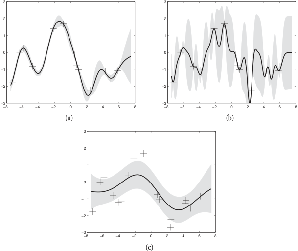
Length scale effect: prior and posterior samples

Short $\ell = 0.1$
Prior

Short $\ell = 0.1$
Posterior

Long $\ell = 5$
Prior

Long $\ell = 5$
Posterior

Top: prior samples. Bottom: posterior samples on the same data.
Short $\ell$: function values decorrelate within tiny gaps → wiggly draws, bands re-inflate between every pair of points.
Long $\ell$: strong long-range correlation → smooth draws, narrow bands — confident even far from data (possibly overconfident).

This is the previous slide’s message shown in the raw material — sample functions, not just summary bands. Left column: at $\ell = 0.1$ the prior draws are noise-like, and the posterior draws only agree in a hair-thin neighborhood of each observation; one step away, the data has no opinion. Right column: at $\ell = 5$ every draw is a lazy arc, and a handful of points pins the function down over the entire domain.
The dangerous panel is the bottom-right and worth dwelling on: long-$\ell$ confidence far from data is a prior assumption, not evidence. The narrow band says “I assumed long-range smoothness,” not “I measured this region.” If the true signal has short-range structure, this model is confidently wrong — the exact failure mode the calibration section audits later.
Practical takeaway to dictate: when a GP’s bands look suspiciously tight, check the fitted length scale against domain knowledge first — it is the single most common cause of overconfident GPs in practice.

Interactive: explore GP kernels and hyperparameters

GP: computational cost

Training: $O(N^3)$ for matrix inversion + $O(N^2)$ storage.
Prediction: $O(N)$ per test point (after training).
Practical limit: $N \approx 10^3 - 10^4$ for exact GPs.
Approximations exist for larger datasets: sparse GPs, inducing points, random features.

Be blunt about why this matters: this single slide is the reason GPs are not the universal default and why the rest of the lecture exists. The $O(N^3)$ comes straight from the matrix inverse in the posterior formula — point back to that box so the cost feels derived, not asserted.
Reframe the limit as a feature for this audience: $N \approx 10^3$–$10^4$ is exactly the regime of expensive experimental materials datasets. GPs are not a weak method that fails at scale — they are the right method precisely where data is scarce and each point is costly. Pair this with the active-learning slide: small-data + uncertainty-guided acquisition is the GP’s home turf.
Mention sparse/inducing-point GPs by name only — “this is how you push to $10^5$+, it’s a known engineering path” — but it is out of scope and the first thing to cut for time. Don’t derive it.

GP: strengths and limitations

Strengths

Principled uncertainty quantification
Automatic complexity control (evidence)
Interpretable hyperparameters
Works well with small data

Limitations

$O(N^3)$ training cost
Kernel design requires domain knowledge
Gaussian assumption may be limiting
Scales poorly to high-dimensional inputs

Use this as the honest scorecard that closes the GP block — don’t oversell. Each strength has a matching weakness, and the engineering lesson is that this profile dictates when to reach for a GP, not whether GPs are “good.”
“Interpretable hyperparameters” is the underrated strength for this cohort: $\ell$ is a length in input units a metallurgist can sanity-check (“correlation over ~50 K of temperature — does that match physics?”). A deep net has no such inspectable knob. That interpretability is a real engineering asset, not a footnote.
The honest weakness to dwell on is “kernel design requires domain knowledge” — there is no free lunch; the RBF default fails on signals with kinks or discontinuities. This sets up the pivot: “When data is large, high-dimensional, or you can’t hand-design a kernel, you switch to neural approaches — and pay for it with approximate, not exact, uncertainty. That is the rest of the lecture.”

Checkpoint: GP prediction

Question: A GP is trained on 10 data points. You query a point very far from all training data. What happens to the uncertainty?
Answer: The posterior variance grows toward the prior variance $\sigma_f^2$. The GP honestly reports high uncertainty in unexplored regions.

Poll it: hands up before reveal. The single most common wrong answer is “the uncertainty stays small because it was trained well” — that is the plug-in-NN mental model leaking in, and catching it here is the whole point of the checkpoint.
Push for the mechanism, not just the answer: as $\mathbf{x}^*$ moves away, $\mathbf{k}_* \to 0$, the subtracted term in the variance formula vanishes, and $\sigma^{*2} \to k(\mathbf{x}^*,\mathbf{x}^*) = \sigma_f^2$. Make them recite the formula’s behavior, not just the slogan — that is the exam-grade answer.
Close the GP block with the one-sentence thesis to carry forward: “A GP is the gold standard for honest uncertainty because the variance formula forces it to admit ignorance away from data. Every method we see next is a cheaper attempt to imitate this without the $O(N^3)$ bill.”

Mixture-Density Networks (MDNs)

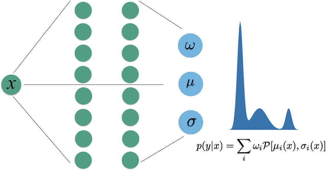
A standard NN outputs a single $\hat{\mathbf{y}}$ (or $\hat{y}$). An MDN outputs parameters of a mixture of Gaussians:

\[ p(\mathbf{y}|\mathbf{x}) = \sum_{k=1}^{K} \pi_k(\mathbf{x}) \, \mathcal{N}(\mathbf{y} | \boldsymbol{\mu}_k(\mathbf{x}), \sigma_k^2(\mathbf{x})) \]

The network predicts mixing coefficients $\omega$, means $\mu$, and variances $\sigma$ — all functions of input $\mathbf{x}$ (Neuer et al. 2024).

MDN architecture: the network outputs $\omega$, $\mu$, $\sigma$ that parameterize a mixture distribution over $y$. (Neuer et al. 2024, fig. 6.10)

Mark the change of philosophy explicitly: GP/MC-Dropout/ensembles infer a distribution; an MDN is just told to output the parameters of one. The network’s last layer emits $(\pi,\mu,\sigma)$ instead of $\hat y$, and you train it by maximizing the mixture likelihood instead of minimizing MSE. This is the “Direct prediction” row of the taxonomy — point back to it.
The “aha” that motivates the whole MDN idea: an ordinary regression NN can only ever say “the answer is around one value” because squared-error assumes a single Gaussian. Some inputs genuinely have two right answers — and a single-Gaussian model is forced to put its mean in the empty valley between them, the one place the truth never is. The next slide shows exactly that failure.
Practical caveat to flag for the bonus exercise: MDN training is finicky (mode collapse, $\sigma\to 0$ blow-ups) — softplus on $\sigma$, enough components $K$. Mention it now so their bonus task isn’t a surprise.

MDN: capturing multi-modal uncertainty

Standard regression assumes unimodal output distribution.
MDNs can represent branching predictions: “this composition could yield phase A or phase B.”
The number of mixture components $K$ is a design choice.
Particularly useful for inverse problems with multiple solutions.

Sell this with the materials story, because it is genuinely their problem: the same alloy composition, depending on cooling path, lands in phase A or phase B. A standard NN predicts the average of the two phase properties — a value that corresponds to no physically realizable material. The MDN reports “60% A, 40% B” with two separate means. That is not a nicer error bar; it is a categorically more correct answer.
“Inverse problems with multiple solutions” is the deep reason and worth one sentence: many materials-design questions (“which composition gives this property?”) are one-to-many by physics. Unimodal regression is structurally wrong for them; multimodality is mandatory, not optional.
Honest limitation: $K$ is a hyperparameter you must guess, and the GP’s automatic complexity control does not come along for free here. Contrast it explicitly — the MDN buys flexibility and gives up the principled model selection of the Bayesian section.

MC Dropout for uncertainty estimation

Standard dropout: randomly zero neurons during training.
MC Dropout: keep dropout active at test time.
Run $T$ stochastic forward passes → $T$ predictions $\{\hat{y}_1, \dots, \hat{y}_T\}$.
Mean = prediction. Variance across samples ≈ epistemic uncertainty.

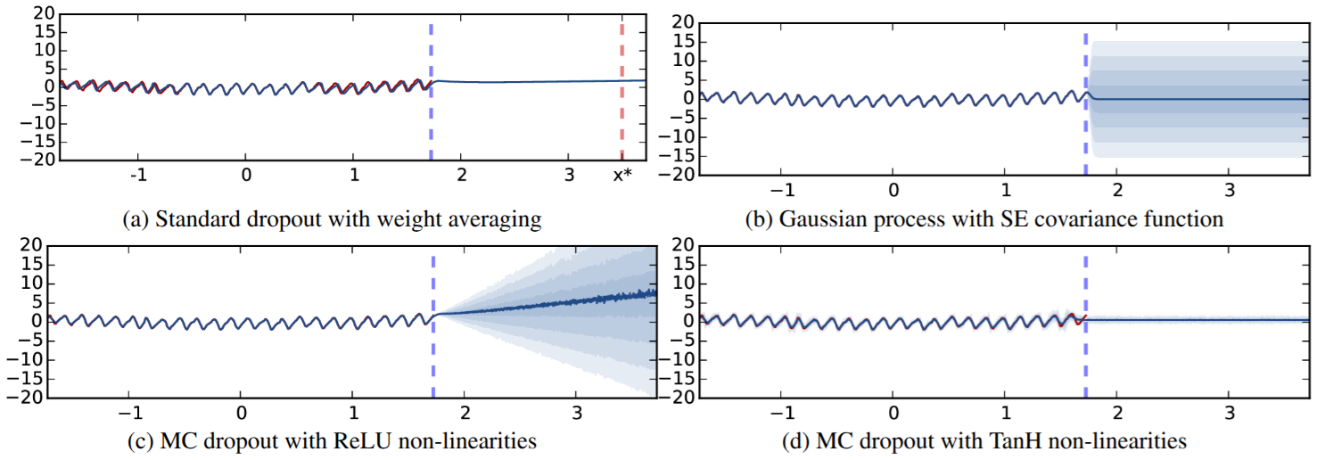
MC Dropout predictive uncertainty on the Mauna Loa CO$_2$ dataset. Red = predictive mean; shaded = uncertainty band. Standard dropout (a) underestimates; MC Dropout with ReLU (c) grows uncertainty outside training range. (Gal and Ghahramani 2016, fig. 2)

The hook that always lands: dropout was invented as regularization — Gal’s insight is that not turning it off at test time turns it into an (approximate) Bayesian posterior sampler. Same code, one line changed (model.train() at inference), uncertainty for free. Students remember the “one-line change” framing.
Connect the figure to the Mauna Loa kernel callback from the “Other kernels” slide — same trend+seasonal signal — and to the variance decomposition: the spread across the $T$ passes is an estimate of the epistemic term. Make panel (c) the focus: outside the training range the band grows, the honest behavior we demanded of every method.
The honest caveat, stated before the next slide makes it precise: MC Dropout’s bands are approximate and notoriously sensitive to the dropout rate — too low and it is overconfident (panel a). It is the cheap imitation of the GP, not an equal. This is exactly the kind of bar the calibration section will teach them to audit before trusting.

MC Dropout: interpretation

Each forward pass uses a different randomly thinned network.
Equivalent to sampling from an approximate posterior over network architectures.
Theoretical connection to variational inference (Gal and Ghahramani 2016).
Advantage: zero additional training cost — uncertainty is free at test time.

Give the one-sentence theory, no more: dropout-at-test is mathematically a variational approximation to a Bayesian neural network — the dropout mask is the variational distribution. State it as “there is a real proof here (Gal & Ghahramani 2016); the takeaway is that this hack is principled, not a trick.” Depth of the VI derivation is out of scope — say so explicitly so nobody waits for it.
The decisive engineering point is the last bullet: zero extra training cost. Versus a deep ensemble’s $M\times$ training bill (next slide), MC Dropout’s only cost is $T$ forward passes at inference. For a model already in production, it is the lowest-friction way to get some uncertainty. Frame the whole MC-Dropout / ensemble pair as a cost-vs-quality decision.
Set up the comparison: “MC Dropout — cheap, approximate, sensitive to dropout rate. Next: deep ensembles — expensive, but the best-calibrated thing that actually scales.”

Deep ensembles

Train $M$ independent networks (different random initializations, same architecture).
Each network produces a prediction $\hat{y}_m$.
Mean: $\bar{y} = \frac{1}{M}\sum_m \hat{y}_m$. Variance: $\frac{1}{M}\sum_m (\hat{y}_m - \bar{y})^2$.
Empirically produces well-calibrated uncertainties. Cost: $M\times$ training (Lakshminarayanan et al. 2017).

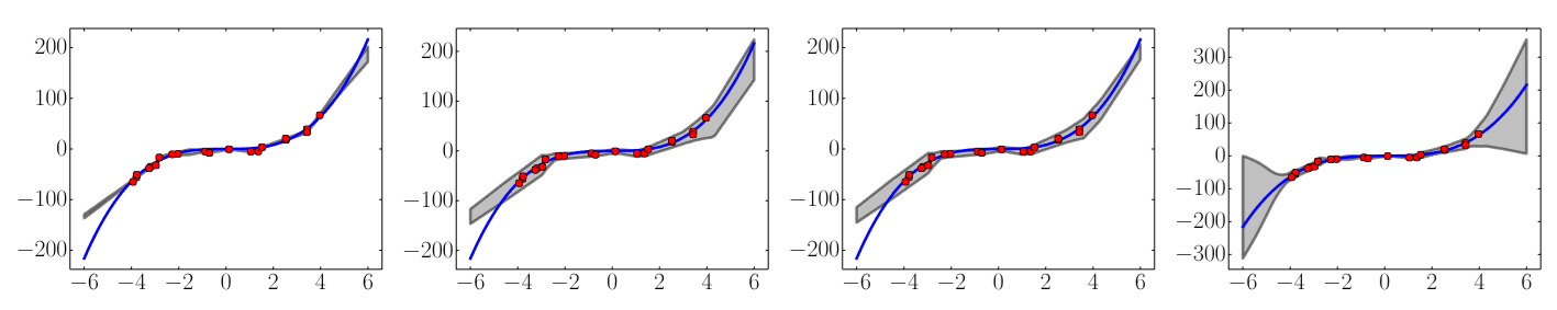
Results on a toy regression task: x-axis denotes x. On the y-axis, the blue line is the ground truth curve, the red dots are observed noisy training data points and the gray lines correspond to the predicted mean along with three standard deviations. Left most plot corresponds to empirical variance of 5 networks trained using MSE, second plot shows the effect of training using NLL using a single net, third plot shows the additional effect of adversarial training, and final plot shows the effect of using an ensemble of 5 networks respectively. (Lakshminarayanan et al. 2017, fig. 1)

The honest headline: this is the embarrassingly simple method that, empirically, wins on calibration — often beating fancier Bayesian approximations. Tell students that plainly; it is a useful corrective to the assumption that more mathematical machinery means better uncertainty.
The mechanism is the variance decomposition’s epistemic term made literal: different random inits → different solutions in the non-convex loss landscape (callback to Unit 6) → they agree near data and disagree in the gaps. The variance across members IS the epistemic uncertainty. Walk the figure panels: the bare MSE ensemble already fans out off-data; NLL + adversarial training sharpens it — same honest behavior the GP gave us, from five for-loop trainings instead of a kernel.
The cost is the whole story for deployment: $M\times$ training (typically $M{=}5$). Position it in the trade-off space — GP: exact but $O(N^3)$; ensemble: scalable and best-calibrated but $5\times$ compute; MC Dropout: cheapest but roughest. That triangle is the examinable summary.

Stochastic enrichment

Add noise to inputs during prediction: $\tilde{\mathbf{x}} = \mathbf{x} + \boldsymbol{\epsilon}$, $\boldsymbol{\epsilon} \sim \mathcal{N}(\mathbf{0}, \boldsymbol{\Sigma}_\epsilon)$.
Run multiple predictions with different noise realizations.
High variance across perturbed predictions = model is sensitive = high uncertainty.
Matches real-world measurement noise propagation (Neuer et al. 2024).

Distinguish it sharply from MC Dropout — students conflate them. MC Dropout perturbs the model (which network). Stochastic enrichment perturbs the input (which measurement). They answer different questions: “how unsure am I about the function” vs “how does my known sensor noise propagate to the output.” Both are Monte Carlo over forward passes; the noise enters in a different place.
Why this is the materials-engineer’s uncertainty, per Neuer: the perturbation covariance $\boldsymbol\Sigma_\epsilon$ is not a tuning knob — it is your measured instrument error bar. This is honest error propagation through a learned model, the ML analogue of propagating measurement uncertainty in a lab. That physical grounding is its main selling point.
Read the figure as sensitivity analysis: uncertainty balloons in the high-$x$ region because the learned function is steep there, so the same input jitter produces a bigger output swing. It surfaces where the model is fragile to measurement noise — complementary to, not a substitute for, epistemic methods.

Calibration: are uncertainties trustworthy? (recall Unit 7)

A model is well-calibrated if predicted $p$% confidence intervals contain $p$% of test points.
Calibration plot: predicted confidence level vs observed coverage.
Perfect calibration = diagonal line.
Overconfident: intervals too narrow (common in NNs). Underconfident: intervals too wide.
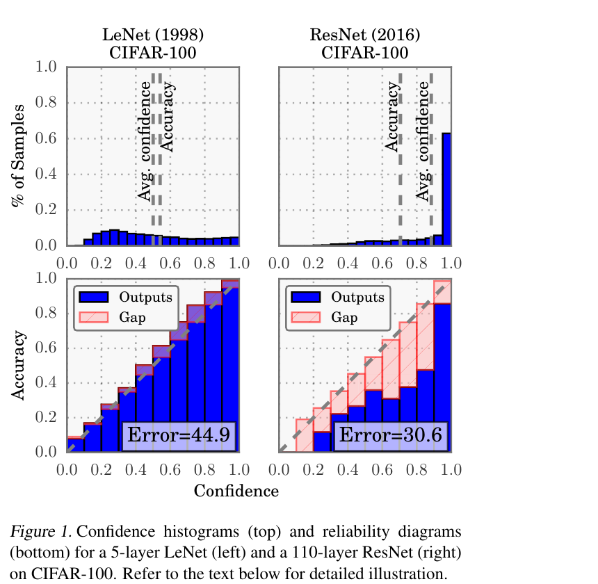
Modern deep NNs are systematically overconfident — confidence exceeds accuracy (Guo et al. 2017).

Reliability diagrams for LeNet (left) and ResNet (right) on CIFAR-100. Blue bars = observed accuracy per confidence bin; gap (pink) shows overconfidence. (Guo et al. 2017, fig. 1)

This slide is the auditor of the entire lecture — make that its job explicit. Every method so far produces an uncertainty number; this is the only tool that asks “is that number true?” An uncalibrated ±10 is a lie with a decimal point. A model can have great accuracy and worthless uncertainty.
The Guo et al. result is the one to state forcefully because it overturns a default assumption: modern deep nets are systematically overconfident, and it got worse as networks got more accurate (LeNet → ResNet). Higher accuracy did not buy honesty — it bought louder wrongness. Connect straight to the “overconfident is the dangerous failure mode” moral from slide 3.
Operational definition for the exam, dictate it: “well-calibrated ⇔ the 90% interval contains the truth 90% of the time, empirically, on held-out data.” The reliability diagram is just that statement plotted; the pink gap is the overconfidence.

Recalibration methods

Temperature scaling: divide logits by a learned temperature $T$ before softmax.
Platt scaling: fit a logistic regression on validation predictions.
Isotonic regression: non-parametric calibration mapping.
Applied post-hoc on a held-out calibration set — does not change the model.

The reassuring engineering message: you do not retrain to fix calibration. These are cheap post-hoc patches fit on a small held-out set, and temperature scaling — a single scalar $T$ — fixes most of the overconfidence in the previous slide’s figure. One number, one validation pass. Lead with that; it is the practical takeaway.
State the honest limitation plainly: recalibration adjusts the model’s stated probabilities and works on average on the calibration distribution — it carries no formal per-prediction guarantee and degrades under distribution shift. “Calibrated” must not be heard as “certified”; for a regulated setting, the calibration audit is evidence, not a proof.
“Does not change the model” is the deployment selling point: certified weights stay frozen, calibration is a thin wrapper — exactly what a safety/QA process wants. One sentence, then move to the synthesis table.

Comparison of UQ methods

Method	Type	Cost	Calibration	Scalability
GP	Exact Bayesian	$O(N^3)$	Excellent	Small $N$
MC Dropout	Approx. Bayesian	$T \times$ inference	Good	Any
Deep ensemble	Frequentist	$M \times$ training	Very good	Any
MDN	Direct	1× training	Requires tuning	Any

Checkpoint: choosing a UQ method

Small dataset, need exact UQ: Gaussian Process.
Large dataset, budget for training: deep ensemble.
Large dataset, need cheap inference: MC Dropout.
Multi-modal outputs: Mixture-Density Network.
Safety-critical decision: whichever method you choose, audit its calibration on held-out data before trusting the bars.

Run this as rapid-fire scenarios, not a slide to read: pose each situation as a one-liner (“50 tensile tests, need honest bars for a design review — go”), let the room answer, then reveal. This is the format their exam question will take, so rehearse the reasoning, not the memorized pairs.
Push past the lookup answer to the why: “small data → GP” is right because GPs are data-efficient and exact and $N$ is small enough that $O(N^3)$ doesn’t bite — all three conditions, recited. A student who says “GP” without the reason hasn’t learned the unit.
The decisive professional habit to leave them with: the last bullet applies on top of whichever method the scenario picked — choosing a method and verifying its calibration are two separate steps, and skipping the second is how overconfident models reach production. That habit is the thesis of the whole second half of the unit.

Materials example: GP for composition-property mapping

GP regression from alloy composition (5 features) to yield strength.
50 training samples from expensive tensile tests.
GP provides uncertainty bands → compositions with high uncertainty are targets for next experiments.
Active learning with GP uncertainty reduces required experiments by 40%.

GP point predictions with 95% credible set: the band narrows at training points and widens in unexplored regions — exactly the signal that guides the next experiment.

This is where the abstract machinery becomes their job — present it as a real workflow, not an illustration. 50 samples, 5-dimensional composition space, each data point a destroyed specimen and a day in the lab. This is the exact $N$, $d$, and cost regime the GP cost slide said GPs own — close that loop explicitly.
The “40% fewer experiments” number is the headline that should make a materials student sit up: the uncertainty band is not a report artifact, it is an experiment-selection device — and translating “I don’t know here” into “so synthesize here next” is worth real money and months. Don’t let it pass as a bullet; it is the practical thesis of the unit.
Honest scope note: 5D is comfortable for a GP; remind them the high-dimensional weakness from the strengths/limitations slide is why this doesn’t trivially extend to a 50-descriptor featurization. Sets up the next slide’s loop and its limits.

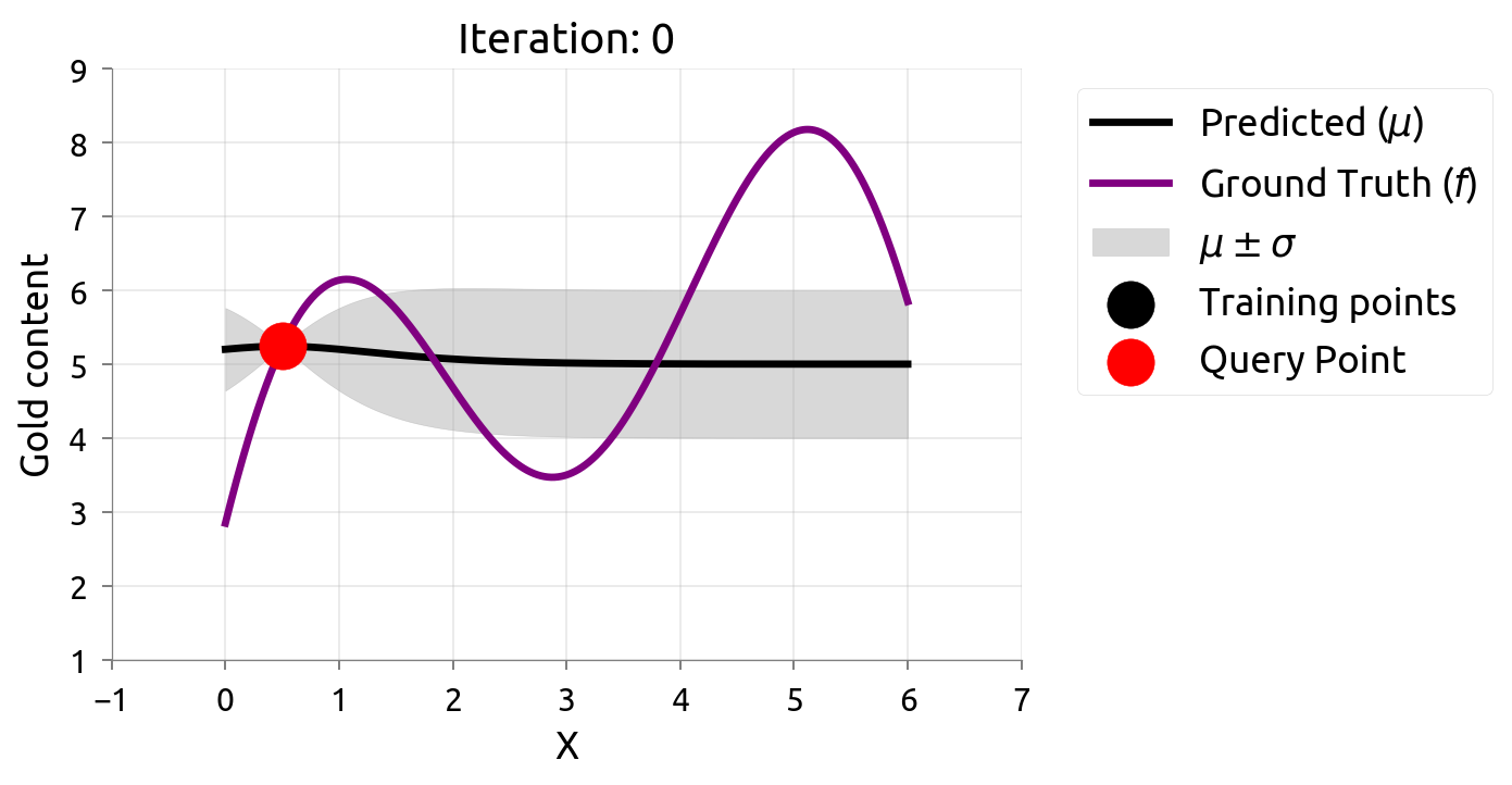
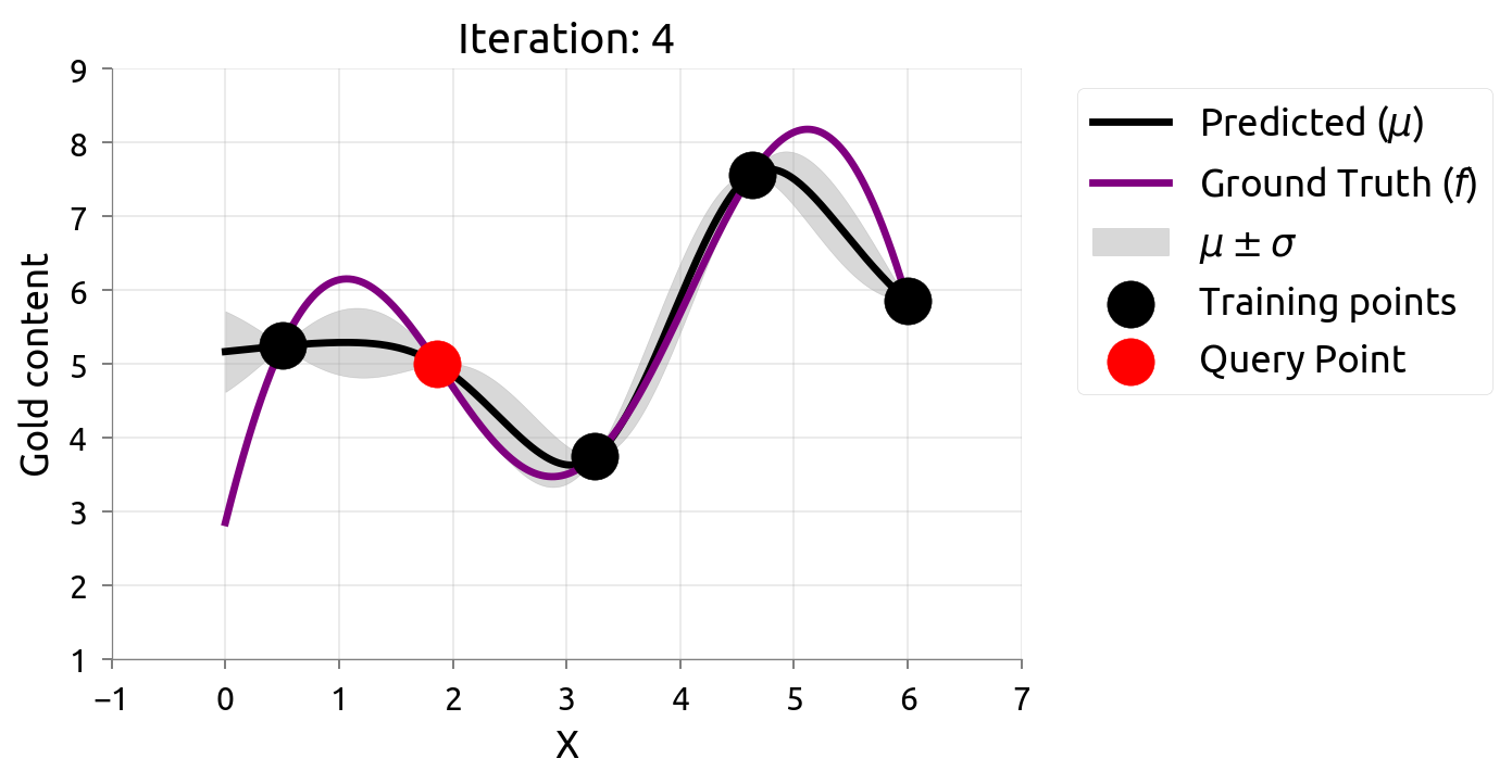
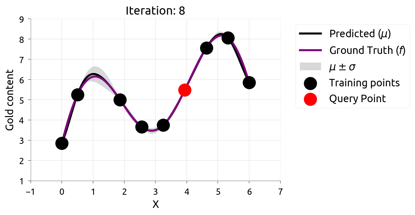
Materials example: active learning with GP uncertainty

Goal: map the composition-property landscape with minimum experiments.
Strategy: train GP, identify input with highest posterior variance, synthesize and test it.
Iterate: retrain GP, select next experiment, repeat.
This uncertainty-driven loop is active learning — the goal is an accurate map of the whole function.

Active learning with a GP surrogate: iterations 0 → 4 → 8. Each round queries the point of maximum posterior variance; the band collapses where data is added and the loop attacks the widest remaining gap.

This is the intellectual peak of the unit — the moment the variance formula becomes an action. Recall the boxed result from the GP-posterior slide: the predictive variance depends only on where you sample, not on $\mathbf{y}$. So you can compute the variance at an unseen composition before synthesizing it — and deliberately go make the most informative experiment. Say this slowly; it is the deepest idea in the lecture.
Walk the three panels top to bottom as the animation: initial GP with huge bands → the loop queries the widest gap → by iteration 8 the band has collapsed nearly everywhere. “Watch the band collapse where we add a point and stay wide elsewhere; the algorithm always attacks the widest gap.”
Name the loop precisely and don’t call it Bayesian optimization yet: max-variance selection is active learning (uncertainty sampling) — pure exploration, aimed at learning the whole function. When the goal is instead finding the best composition, exploration must be traded against exploitation — that is Bayesian optimization, next slide. Students (and papers) conflate the two constantly; this unit doesn’t.

From active learning to Bayesian optimization

Active learning: map the function accurately → acquire at max variance (pure exploration).
Bayesian optimization: find the maximum with fewest experiments → acquisition must balance exploitation (high mean) against exploration (high variance).
Expected Improvement over the best value $f^+$ observed so far:

\[ \mathrm{EI}(\mathbf{x}) = \left(\mu(\mathbf{x}) - f^+ - \epsilon\right)\Phi(Z) + \sigma(\mathbf{x})\,\phi(Z), \quad Z = \frac{\mu(\mathbf{x}) - f^+ - \epsilon}{\sigma(\mathbf{x})} \]

$\epsilon$ dials exploration ↔︎ exploitation. Alternatives: probability of improvement, UCB $\mu + \beta\sigma$, Thompson sampling.

Both loops are the engine of self-driving labs and autonomous microscopy.
Same GP machinery, different acquisition function — the acquisition is the experimental strategy.
Deep dive with iteration-by-iteration visualizations: Data Science for EM, Units 6–7.

The one distinction to leave the room with: active learning asks “where do I know least?”, Bayesian optimization asks “where is the best candidate likely hiding?” — and the entire difference is the acquisition function. The GP underneath is identical; you swap one formula and get a different scientific instrument.
Read EI’s two terms as the trade-off made explicit: the first term is large where the mean already beats the incumbent $f^+$ (exploitation); the second is large where $\sigma$ is big (exploration). $\Phi$ and $\phi$ are just the Gaussian CDF/PDF of the standardized improvement — no new machinery, everything comes from the GP posterior of this lecture.
Don’t derive EI — state it and interpret it. If a student wants the derivation and the ε-sweep animations (what happens with too much exploration), point them at the DSEM course units 6–7, which walk PI/EI/Thompson iteration by iteration on the same kind of 1-D toy problem.
Close the loop to the unit thesis: the acquisition function is uncertainty acted upon. A model that cannot say “I don’t know here” cannot run this loop at all — honest UQ is not a reporting nicety, it is the prerequisite for autonomous experimentation.

Lecture-essential vs exercise content split

Lecture: Bayesian prediction, evidence framework, GP derivation, practical UQ taxonomy, calibration.
Exercise: GP implementation from scratch, kernel hyperparameter exploration, ensemble comparison, MDN bonus.

Exercise setup summary

Implement GP regression (RBF kernel) in NumPy: compute posterior mean and variance.
Compare GP uncertainty bands with predictions from an NN ensemble (3 networks).
Vary length scale $\ell$ and observe effect on fit and uncertainty.
Bonus: implement a simple MDN with 2 Gaussian components in PyTorch.

Frame the exercise as “make the closed-form slide real with your own hands”: the GP task is literally typing the two boxed posterior formulas into NumPy — ~15 lines, one np.linalg.solve, no library. The point is to feel that the honest uncertainty bands fall directly out of that algebra, with nothing hidden in a .fit() call.
Pre-empt the two predictable stumbles so office hours aren’t swamped: (1) numerical instability inverting $\mathbf{K}$ — tell them now to add a jitter term $\sigma_n^2\mathbf{I}$, which is also the physically meaningful noise term, not a hack (connect to the conditioning slide); (2) the length-scale sweep should reproduce the length-scale-effect figure — if their short-$\ell$ run isn’t wiggly with exploding between-point bands, they have a bug.
Position the GP-vs-ensemble comparison as the experiment that earns the whole comparison table: same data, see for themselves that two completely different methods both fan out off-data — that convergence is the unit’s central empirical claim, not just a slide.

Exam-aligned summary: 10 must-know statements

The Bayesian predictive distribution integrates over parameter uncertainty.
Total prediction variance = aleatory variance + epistemic variance.
The marginal likelihood (evidence) measures model fit with automatic complexity penalty.
A GP is a distribution over functions specified by mean and kernel functions.
The GP posterior has closed-form mean and variance (for Gaussian likelihood).
GP uncertainty grows away from training data — honest epistemic uncertainty.
Kernel hyperparameters (length scale, signal variance) control GP behavior.
MC Dropout approximates Bayesian inference by sampling sub-networks at test time.
Deep ensembles provide uncertainty via disagreement among independently trained models.
Calibration plots verify that predicted confidence matches observed accuracy.

This is the contract from the learning-outcomes slide, closed. Read each statement and, in one breath, name the slide it came from — students should see the lecture replay as a 10-beat spine. If a statement doesn’t trigger recognition, that is their personalized revision list; tell them to self-audit live.
Flag the three that are derivation questions, not recall: #2 (write the law-of-total-variance split and name each term), #3 (the evidence integral + the Occam argument), #5 (reproduce both boxed GP posterior formulas). The other seven are explain-in-two-sentences. Make the format expectation explicit so revision is targeted.
The one-sentence thesis to end on, said slowly: “A prediction without a defensible uncertainty is not an engineering result. This unit gave you the principled version (GP), the scalable versions (dropout, ensembles, MDN), and the auditor (calibration). Knowing which to deploy for a given decision is the actual skill.” Then hand to the exercise.

Continue

← Previous: Unit 11 — Generative Models — VAE & Diffusion
→ Next: Unit 13 — Physics-Informed & Constrained Learning
All courses

References + reading assignment for next unit

Required reading before Unit 13:
- Murphy: Ch. 5, 15
- Neuer: Ch. 6.4
Optional depth:
- Bishop: Ch. 3.5 (evidence framework)
- Rasmussen & Williams: GP reference text
Next unit: Physics-Informed Learning — embedding domain knowledge into ML models.

Make the reading purposeful, not a list: Murphy Ch. 5 is the evidence/empirical-Bayes block and Ch. 15 is the GP block — reading them before Unit 13 closes the gaps this 90 min compressed (the eigen-decomposition behind effective parameters; the sparse-GP scaling we name-dropped). Tell them which slide each chapter back-fills.
Sell Rasmussen & Williams as the one reference to actually own if they do anything Bayesian later (thesis, ML-PC course) — it is the GP text and freely available online; the GP exercise will make Ch. 2 readable in an afternoon.
One-line bridge to Unit 13, stated as a question to carry out the door: “Today physics entered only as an informative prior in passing — next unit, how do you build a conservation law into the model itself so the uncertainty tightens without new data?” Leave them with the question, not a summary.

Bishop, Christopher M. 2006. Pattern Recognition and Machine Learning. Springer.

Gal, Yarin, and Zoubin Ghahramani. 2016. “Dropout as a Bayesian Approximation: Representing Model Uncertainty in Deep Learning.” Proceedings of the 33rd International Conference on Machine Learning 48: 1050–59. https://proceedings.mlr.press/v48/gal16.pdf.

Guo, Chuan, Geoff Pleiss, Yu Sun, and Kilian Q. Weinberger. 2017. “On Calibration of Modern Neural Networks.” Proceedings of the 34th International Conference on Machine Learning 70: 1321–30. https://arxiv.org/abs/1706.04599.

Lakshminarayanan, Balaji, Alexander Pritzel, and Charles Blundell. 2017. “Simple and Scalable Predictive Uncertainty Estimation Using Deep Ensembles.” Advances in Neural Information Processing Systems 30. https://papers.nips.cc/paper_files/paper/2017/hash/9ef2ed4b7fd2c810847ffa5fa85bce38-Abstract.html.

Murphy, Kevin P. 2012. Machine Learning: A Probabilistic Perspective. MIT Press.

Neuer, Michael et al. 2024. Machine Learning for Engineers: Introduction to Physics-Informed, Explainable Learning Methods for AI in Engineering Applications. Springer Nature.

Tran, Kevin, Willie Neiswanger, Junwoong Yoon, Qingyang Zhang, Eric Xing, and Zachary W. Ulissi. 2020. “Methods for Comparing Uncertainty Quantifications for Material Property Predictions.” Machine Learning: Science and Technology 1 (2): 025006. https://arxiv.org/abs/1912.10066.

Approach	Output	Uncertainty	Cost
MLE/MAP	Single \(\hat{\mathbf{y}}\)	None (or ad-hoc)	Low
Bayesian (exact)	Full \(p(\mathbf{y}^\|\mathbf{x}^,\mathcal{D})\)	Principled	High
Bayesian (approx.)	Approximate distribution	Approximate	Moderate

Method	Type	Cost	Calibration	Scalability
GP	Exact Bayesian	\(O(N^3)\)	Excellent	Small \(N\)
MC Dropout	Approx. Bayesian	\(T \times\) inference	Good	Any
Deep ensemble	Frequentist	\(M \times\) training	Very good	Any
MDN	Direct	1× training	Requires tuning	Any

Mathematical Foundations of AI & MLUnit 12: Uncertainty in Predictions