Machine Learning in Materials Processing & Characterization
Unit 3: Data Quality, Preprocessing, and Robust Validation

Prof. Dr. Philipp Pelz

FAU Erlangen-Nürnberg

01. Where We Are

Recap — Units 1 & 2

• Unit 1: materials data is small, expensive, hierarchical, and probe-dependent.
• Unit 2: the measurement chain \(\xi(t)\rightarrow x_i\) — every datum is a sample of a physical process plus noise.

Today — Unit 3

The data has arrived in your computer. What now?

• It is messy, mis-scaled, partly missing, and inconsistently labelled.
• Before any model: clean, transform, validate.
• Before believing any score: rule out leakage.

Position the unit. Unit 1 told us what materials data looks like, Unit 2 told us how it is generated by a physical sensing chain. Unit 3 is where we close the gap between the raw file the instrument hands us and the well-behaved tensor a model can train on. It is also the unit where students learn the discipline that separates a publishable result from a spurious one.

Set expectations. Preprocessing and validation are unglamorous. They are also where 80% of project time goes in industry, and where almost all of the “ML doesn’t work for our data” stories actually originate. Tell students explicitly: this is the unit that will save their thesis.

Connect to later units. The skills from today reappear in: - Unit 6 (transfer learning — when scarce data forces clever validation) - Unit 7 (time series — temporal leakage, triggering) - Unit 8 (generalization & robustness — group splits, distribution shift) - Unit 12 (uncertainty / GPs — Bayesian posteriors first introduced today)

02. Learning Outcomes

By the end of this lecture, you will be able to:

1. Diagnose common data-quality problems (missing values, outliers, duplicates, scale mismatch) and choose appropriate repair strategies.
2. Apply standard transformations — centering, standardization, log, differentiation, FFT, wavelet — and explain why each is needed for a given algorithm.
3. Distinguish noise outliers from rare physical events using domain knowledge.
4. Quantify label uncertainty (inter-annotator variance, soft labels) and explain the Bayesian prior–likelihood–posterior view.
5. Design robust validation (k-fold, stratified, group-based, time-aware) that prevents data leakage.
6. Choose the right error metric for a regression or classification task in materials science (MAE/RMSE/\(R^2\) vs. precision/recall/IoU/Dice).

Bloom mapping. Outcomes 1, 2, 5, 6 are at the apply / analyse level — students should be able to walk into a project and execute. Outcomes 3 and 4 are at the evaluate level: judging whether a thing is an artifact or signal, deciding whether labels are trustworthy.

Assessment hook. Tell students which exercises in the problem set map onto which outcome. Outcome 5 is heavily exam-relevant — leakage is the most common reason published ML papers in materials science fail to reproduce.

03. The Running Headline — GIGO

“On two occasions I have been asked, ‘Pray, Mr. Babbage, if you put into the machine wrong figures, will the right answers come out?’ I am not able rightly to apprehend the kind of confusion of ideas that could provoke such a question.” — Charles Babbage, 1864

Garbage In, Garbage Out (GIGO): model accuracy is bounded by data quality before any architectural choice.

A representative materials-science failure mode:

• A CNN trained on TEM images of nanoparticles reports 94% accuracy.
• It actually learned to detect the carbon-grid pattern — present in 94% of “particle” images and 0% of “no-particle” images.
• No architecture fix would have helped. Only data hygiene would.

The hook. Open with the Babbage quote — students enjoy it, and it sets the tone that this is a centuries-old discipline, not a new ML annoyance. Then drop the carbon-grid example. This is a true family of failures (the “Husky vs Wolf”–style shortcut, transferred to TEM).

Drive home the asymmetry. Spending another week on hyperparameter search will not recover from a data leak. Spending an hour on data cleaning often turns a 60% model into a 90% model. Make the implicit ROI argument explicit.

Connect forward. When we discuss explainability and saliency maps in later units, the carbon-grid story comes back as Exhibit A for why you need attribution methods to catch silent failures.

04. The ML Workflow Through Today’s Lens

The classical pipeline (CRISP-DM, Unit 1):

1. Data collection — Unit 2.
2. Data preprocessing — today, §1–§3.
3. Model training — Units 4–7.
4. Validation — today, §4–§5.
5. Deployment & monitoring.

Steps 2 and 4 typically dominate calendar time on real projects.

Today’s structure

• §1 Cleaning (≈14 min)
• §2 Transformations & scaling (≈22 min)
• §3 Labels & uncertainty (≈9 min)
• §4 Bias–variance & regularization (≈8 min)
• §5 Validation & leakage (≈14 min)
• §6 Error metrics (≈12 min)

Three short think-pair-share checkpoints along the way.

Signposting. Students orient much better when they know the shape of the lecture. Promise the breaks (active-learning slides) so they pace their attention.

Time-honesty. The transformations section is the longest because it has the most formula content and a worked example. The validation section is the most exam-relevant. The cleaning section is short but conceptually dense.

§1 · Data Cleaning

05. The Measurement Chain — Where Errors Enter

\[ \underbrace{\xi(\tau)}_{\text{physical state}} \;\to\; \text{probe} \;\to\; \text{detector} \;\to\;\\\to\; \underbrace{\text{ADC} \;\to\; \text{file}}_{\text{digital}} \;\to\; \mathbf{x} \]

Errors can enter at every link:

• Sensor: drift, saturation, dead pixels, dark current.
• Transmission: dropped packets, timestamp skew.
• Storage: wrong dtype, units lost in the header.
• Human: transposed columns, mis-labelled batches.

Strategy: clean at the source first.

• A bad sensor produces bad data forever.
• Digital “repair” interpolates — it cannot recover information that was never recorded.
• Always document where in the chain a fix was applied: it changes how downstream models should interpret the data.

Anchor in Unit 2. Remind students the measurement chain \(x_i = \xi(\tau_i + \delta t) + u_x\) introduced in Unit 2 — today we deal with the residual that survives that chain plus purely digital pathologies (typos, NaNs, duplicates).

The “source first” principle. Worked example: a thermocouple reading \(-1273\,°\mathrm{C}\) because the lead wire broke. Two responses: (a) drop the row in pandas — fast, but the broken wire keeps producing bad rows tomorrow; (b) replace the wire — slow, but solves the class of failures. Industrial ML practice strongly prefers (b). Where (b) is impossible (legacy data, sealed instrument, archival), document the digital repair so a reader can recompute without it.

Why explainability cares. If you imputed missing values with column means, every post-hoc explanation tool will see those imputed rows as “typical” — masking exactly the samples that were anomalous in reality.

06. Six Failure Modes You Will Meet

1. Structural problems — typos, mixed units (hPa vs kPa), wrong delimiters, mixed date formats.
2. Duplicates — repeated frames in a video, the same DOE point recorded twice.
3. Irrelevant observations — pre-experiment baseline still in the file.

4. Missing values (NaN) — sensor drop, out-of-range, transmission loss.
5. Outliers — point, contextual, collective (next slide).
6. Mislabelled rows — class flipped, sample ID lost, condition swapped.

Note

Most of these are caught only by visualizing the data. Always plot before fitting.

Practical advice. Open the dataset in pandas, run df.describe(), df.info(), and a small grid of histograms / scatter plots before any modelling. The single most effective “ML technique” in industry is matplotlib.

War story. A common failure: column dtypes silently coerced — temperatures read as strings, sorted lexicographically (“100” < “20”). The model trains, predicts, and ships nonsense. df.dtypes catches it in two seconds.

Materials-specific pitfalls. Mixed units across instruments (kV vs V, Pa vs MPa); sample IDs encoded as integers that get auto-converted to scientific notation in Excel (yes, this is still a problem); time stamps with and without timezone.

07. Missing Values — Repair Options

Where do NaNs come from?

• Sensor saturation or dropout.
• Transmission gap (Bluetooth / Wi-Fi).
• Out-of-range readings (“\(-1273\,°\mathrm{C}\)” stored as NaN by the driver).
• Pandas re-indexing across heterogeneous frames.

Three repair strategies:

1. Drop the row — safe only if NaNs are MCAR (missing completely at random).
2. Interpolate: linear, mean, median, model-based.
3. Mark with an out-of-range numeric token and let the model see “this was missing.”

Linear interpolation between neighbours Neuer, Michael et al., (2024), eq. 3.1: \[ x_i \;=\; \tfrac{1}{2}\bigl(x_{i-1} + x_{i+1}\bigr) \]

Numerical marker (temperature sensor, range \([-50, 100]\,°\mathrm{C}\)): \[ x_i^{\text{NaN}} \;=\; -1000\,°\mathrm{C} \] chosen outside the physically possible range, so downstream code can treat it specially.

Note

Trap. Replacing NaN with \(0\) silently inflates the count of zero-readings and biases statistics.

MCAR / MAR / MNAR taxonomy. Briefly mention: missing completely at random (drops are safe), missing at random (drops bias the dataset along an observable variable, can be corrected), missing not at random (drops bias the dataset along an unobservable variable — often the most interesting case, e.g., the instrument fails because the sample is unusual).

Why markers beat zeros. Zero is a value the sensor can produce. -1000°C is not. A model or feature engineer can build a “was-missing” indicator from the marker. With zero, the information is destroyed.

Connect to imaging. In TEM/SEM, “missing” can mean an entire scan line dropped or a detector quadrant dead. Inpainting (a learning method itself) is the right tool there; interpolation suffices only for sparse, isolated NaNs.

08. Outliers — Three Flavours

Point / global outlier. A single value far from the bulk of the distribution. Tensile test: one stress reading at \(10\,\mathrm{GPa}\) in a \(\sim 500\,\mathrm{MPa}\) dataset.

Contextual outlier. A value that is reasonable globally but anomalous given its neighbours. Time series: a \(300\,\mathrm{K}\) reading inside a furnace ramp at \(1500\,\mathrm{K}\).

Collective outlier. A sub-sequence whose individual values look fine but whose joint behaviour deviates. Stress–strain: an entire curve with the wrong loading rate.

Detection toolbox

• Distribution-based: \(|x - \mu| > k\sigma\), IQR rule, Mahalanobis distance.
• Model-based: residuals from a fit, isolation forests, one-class SVM.
• Density-based: DBSCAN, LOF.
• Visualization: boxplots, scatter, residual plots.

For a tensile-test example, see Figure 11.4 in Sandfeld et al., Materials Data Science.

Materials examples.

• Point: a Hall-effect reading that hit the rail because the field exceeded the probe range.
• Contextual: a XRD intensity that is fine in absolute terms but inconsistent with the background trend in that 2θ window.
• Collective: a fatigue cycle whose load amplitude was wrong by a factor of 10 — every individual reading is plausible, the cycle is not.

Why the taxonomy matters. Different detection methods catch different kinds. A z-score test catches points; you need temporal models for contextual, and sequence models for collective.

Anti-pattern. Don’t drop outliers based on a single statistical test without looking at them. The first material that ever passed superconductivity Tc would have been a 6-sigma outlier in any prior dataset.

09. Outlier or Rare Event? The Crucial Decision

A point well outside the distribution may be:

• Artifact → measurement noise, ADC saturation, sample contamination → remove.

• Rare physical event → crack initiation, phase nucleation, beam damage onset → keep, perhaps weight up.

The decision is not statistical. It is physical.

Heuristic checklist before removing a point

1. Reproduce: do nearby measurements show the same trend?
2. Cross-instrument: does another sensor agree?
3. Process log: was anything unusual recorded?
4. Domain plausibility: is it physically possible?
5. Consequence: how would the downstream model change if it were real?

Default rule of thumb: flag, don’t drop. Keep an “outlier” column. Train with and without; report both.

Pause-and-discuss prompt. Show a stress–strain curve with one anomalously high stress peak and one anomalously low one. Ask: which would you remove? Neither, until you know the experiment. The high peak might be a Lüders band; the low one might be a slipped extensometer.

War story. The discovery of the Higgs boson lived as a 5σ outlier in a sea of pure noise — for years it was indistinguishable from background. Materials analogues: defect nucleation events in fatigue testing, single-photon avalanche events in detectors, beam damage onset in cryo-EM.

Connect to Unit 8. “Distribution shift” and “process windows” formalise the intuition that the region where rare events occur is also the region where models extrapolate worst — exactly where keeping rare events is most valuable.

10. Duplicates — Quiet but Damaging

Sources

• DOE point recorded twice by the operator.
• Frame repeated by a camera at variable rate.
• Same TEM micrograph cropped in two places.
• Database join with one-to-many cardinality.

Why it matters

• Statistics: duplicates over-weight the duplicated condition, biasing means and variances.
• ML training: duplicates inflate apparent accuracy.
• Validation: identical rows on both sides of a split → leakage.

Detection idioms (pandas)

df.duplicated().sum()
df.drop_duplicates(subset=["sample_id", "t"])

For images / spectra: exact duplicates miss near-duplicates (different crops, different exposures of the same scene). Use perceptual hashes or learned embeddings.

Materials trap. Many “different” measurements come from the same specimen. They are not duplicates by row, but they are correlated by physics. We will return to this in §5 (group leakage).

Sharpen the distinction. A row-level duplicate is a literal copy. A group duplicate is a set of distinct rows that share an underlying physical entity (a sample, a coupon, a batch). Both inflate validation scores; the second one is harder to detect because df.duplicated() won’t flag it.

Pre-flight for any dataset. (1) df.duplicated().sum() (2) is there a sample_id / specimen_id column? (3) if yes, what is the groupby(sample_id).size() distribution? This last query alone catches many “leaks” before any model is trained.

§2 · Transformations & Scaling

11. Why Transform Data?

Three goals

1. Comparability. Make features with different units directly comparable.
2. Numerical conditioning. Avoid dominance by large-magnitude features in distance- or gradient-based methods.
3. Linearisation. Reveal structure (exponential trends, oscillations, transients) that is hidden in the raw representation.

Algorithms that care about magnitude

• \(k\)-NN and any Euclidean-distance method.
• PCA / SVD (Unit 4) — variance is scale-dependent.
• Gradient descent — different scales → different effective learning rates per parameter.
• Regularised linear models — penalty applies per-coordinate.

Algorithms that don’t (much)

• Decision trees and forests.
• Tree-based gradient boosting.
• Methods using only rank statistics.

A general warning

Transformation is a modelling decision. It changes the effective prior the algorithm sees. Document and motivate every transform you apply §11.5.3 in Sandfeld et al., Materials Data Science.

Tie back to Unit 4. PCA decomposes the covariance of standardized features. Without standardization, PCA is dominated by whatever feature happens to have the largest variance — usually an artefact of units, not physics. We will meet this concretely next week with eigen-microstructures.

Why trees don’t care. A decision tree splits on \(x_j > \tau\). Any monotonic transformation \(x_j \mapsto f(x_j)\) leaves the order intact, hence the same splits are available. Standardising before a random forest is harmless but also useless. Standardising before kNN is essential.

Numerical view. Adam’s per-parameter adaptive scale partially compensates for unscaled features, but ill-conditioned feature matrices still hurt convergence and generalisation.

12. Centering and Shifting

Centering (mean-subtraction): \[ \tilde{x}_i = x_i - \langle x \rangle, \qquad \langle \tilde{x} \rangle = 0 \]

• Required by methods that interpret the origin as a reference (PCA, covariance, FFT phase).
• Preserves the shape of the distribution; only the location changes.

Shifting (alignment): \[ \tilde{x}_i^{(k)} = x_i^{(k)} - x^{(k)}_{\text{ref}} \]

• Align peak positions across spectra, or zero-the-extensometer across tensile curves.

Materials examples

• XRD: shift each pattern so its strongest reflection sits at \(2\theta = 0\) before averaging.
• Stress–strain: shift each curve so the elastic origin coincides — corrects for grip slip.
• Spectroscopy: align a known reference line (e.g., Si Raman peak at \(520\,\mathrm{cm}^{-1}\)).

Caution. Shifting destroys absolute calibration. Keep the offsets if you may need them later (e.g., for absolute energy alignment).

Be precise about what shifting changes. It moves the data; it does not rescale or reshape. The distribution’s spread, skew, and kurtosis are invariant. Useful when the quantity of interest is the shape (peak width, peak ratio, decay rate) rather than the absolute value.

Pitfall. Naive grand-mean centering across a heterogeneous dataset can mask class differences. Center per-group only when the per-group mean is itself uninformative.

13. Min–Max and Range Scaling

Min–max scaling to \([0, 1]\): \[ \tilde{x}_i \;=\; \frac{x_i - \min(\mathbf{x})}{\max(\mathbf{x}) - \min(\mathbf{x})} \]

Variants

• \([-1, 1]\): divide by \(\max(|\mathbf{x}|)\) after centering.
• Sum-normalisation: \(\tilde{x}_i = x_i / \sum_j x_j\) (preserves area; suitable for histograms / spectra interpreted as densities).

Use when

• The feature has a known, bounded range (image pixel intensities \([0,255]\)).
• You need values in a fixed interval for numerical stability (e.g., feeding a bounded activation).

Avoid when

• The data has heavy tails — a single extreme value compresses everything else.
• Min/max change between train and test sets (and they will).

Neuer, Michael et al., (2024), eqs. 3.2 – 3.4

Outlier sensitivity. Min–max is dominated by the most extreme point in the sample. Move one outlier from \(10\) to \(1000\) and every other point gets compressed by 100×. Standardisation (next slide) is dominated by \(\mu\) and \(\sigma\), which are far less fragile.

Train/test discipline. The min and max are parameters of the transform. They are fit on the training set and applied to the test set. Re-fitting on the test set is a form of leakage. We’ll see this systematically in §5.

14. Standardization (Z-Score)

\[ z_i \;=\; \frac{x_i - \mu}{\sigma}, \qquad \mu = \langle x \rangle, \quad \sigma^2 = \langle (x-\mu)^2 \rangle \]

After standardisation: \(\langle z \rangle = 0\), \(\mathrm{Var}(z) = 1\).

Properties

• Robust to scale; less sensitive to outliers than min–max.
• Does not make non-Gaussian data Gaussian (Fig. 11.8 in Sandfeld, Stefan et al., (2024)).
• The default for distance-based methods, PCA, regularised linear models.

Worked example — Motor currents Neuer, Michael et al., (2024)

Problem: a fleet of motors logs current. Some channels record in mA, others in A — three orders of magnitude difference. Raw plot: half the curves look “flat”.

Fix: standardise each curve (or rescale unit families) so all channels share a common axis. The anomalous motor now visibly deviates.

Lesson: the fix is one line of code. The diagnosis required a domain expert and a plot.

Bias–variance for the transform itself. Why divide by \(\sigma\) rather than the range? Range is an extreme-value statistic — non-robust. \(\sigma\) averages over all points and inherits Central-Limit-Theorem stability.

Materials warning. Standardising on the full dataset before train/test split leaks test-set information (the mean and std saw test data). The disciplined recipe: fit \((\mu, \sigma)\) on train, transform train and test using those frozen values. Use scikit-learn’s StandardScaler.fit on train, .transform on both. We will return to this in §5.

Robust alternatives. When the data has extreme outliers, replace \(\mu, \sigma\) with median and interquartile range (RobustScaler).

15. Non-Dimensionalisation — Physics-Aware Scaling

Idea: divide each quantity by an intrinsic physical scale, not a statistical one.

\[ \tilde{x} \;=\; \frac{x}{x_{\text{ref}}}, \qquad x_{\text{ref}} \in \{L_0, T_0, c, k_B, \dots\} \]

Examples

• Strain \(\varepsilon\) is already non-dimensional (\(\Delta L / L_0\)).
• Reynolds number, Péclet number — scaled flow variables.
• Temperatures normalised by \(k_B T / E_{\text{barrier}}\) in Arrhenius analyses.

Why physicists prefer this

• Removes spurious scale dependence — the laws look the same.
• Reveals the true number of independent parameters (Buckingham \(\pi\)).
• Makes ML models that respect known physical symmetries.

Connect: Unit 13 (PINNs) leans heavily on non-dimensionalisation — it is what lets a single trained model generalise across orders of magnitude.

The right scale depends on the problem. For a polycrystal, the natural length scale might be the grain size; for a fatigue specimen, the gauge length; for a TEM image, the pixel size in real space. There is no general recipe — domain knowledge picks \(x_{\text{ref}}\).

Why ML cares. A neural network trained on data scaled by an arbitrary unit choice generalises poorly to a new unit choice. A network trained on non-dimensional inputs is unit-agnostic by construction.

16. The Log Transform

\[ \tilde{x}_i \;=\; \log(x_i + \epsilon), \qquad x_i > 0 \]

Linearises power laws and exponentials.

• \(y = a x^b \;\Rightarrow\; \log y = \log a + b \log x\).
• Arrhenius: \(\log k = \log A - E_a /(k_B T)\).
• Hall–Petch: \(\sigma_y = \sigma_0 + k d^{-1/2}\).

Compresses dynamic range.

• Grain sizes spanning \(10\,\mathrm{nm}\) to \(10\,\mathrm{mm}\) → six decades.
• Dislocation densities, time-to-failure, particle-size distributions.

Practical rules

• Add a small \(\epsilon\) to handle zeros; document its value.
• Do not log-transform variables that can legitimately be zero or negative without first thinking about the physics.
• After log-transform, errors are relative, not absolute — change your loss function (MSLE, log-likelihood) accordingly.

Connect: the MSLE error metric (§6) is the natural error after a log-transform.

Statistical view. A log-transform is the Box–Cox transform with \(\lambda \to 0\). It moves multiplicative noise into the additive regime, which makes Gaussian assumptions realistic. For variables whose noise is genuinely multiplicative — most concentration, intensity, count, and rate measurements in materials science — the log-transform is not optional, it is the correct preprocessing.

Anti-example. Don’t log-transform stress unless you have a good reason; the natural noise on stress is closer to additive Gaussian. Log-transforming it makes things worse.

17. Differentiation as a Convolution

Forward difference as a discrete kernel Neuer, Michael et al., (2024), eq. 3.10: \[ \frac{d\mathbf{f}}{dx} \;\approx\; \mathbf{f} \ast [-1, +1] \]

Second derivative: \[ \frac{d^2\mathbf{f}}{dx^2} \;\approx\; \mathbf{f} \ast [+1, -2, +1] \]

What it does

• Removes constant baselines (DC offset → 0).
• Enhances change points, spikes, transitions.
• Makes anomaly detection easier in slowly drifting signals.

Practical caveat

Differentiation amplifies high-frequency noise. Combine with smoothing in one kernel: \[ \mathbf{f} \ast [-1,-1,-1,-1,+1,+1,+1,+1]/4 \]

(Savitzky–Golay filters generalise this idea.)

Materials applications

• Derivative spectroscopy (Raman, IR) to highlight peak shoulders.
• Strain-rate from displacement.
• Acoustic-emission event detection from continuous load signals.

Why convolution view matters. It tells students immediately that the same operation sits at the heart of CNNs (Unit 5). A first-derivative kernel is a learned edge detector. Edge filters are the simplest possible convolutional features.

Numerical stability. Higher-order finite differences are more sensitive to noise. The Savitzky–Golay polynomial filter fits a low-order polynomial in a moving window and returns its analytical derivative — robust against noise while preserving peaks.

Common mistake. Differentiating the noisy signal first and then smoothing is worse than smoothing first and then differentiating. The order matters because the smoothing filter is not orthogonal to the derivative.

18. From Time to Frequency — the FFT

Continuous Fourier transform Neuer, Michael et al., (2024), eq. 3.14: \[ \hat{x}(\nu) \;=\; \frac{1}{\sqrt{2\pi}}\int x(t)\, e^{-i 2\pi \nu t}\, dt \]

Why we transform

• Periodic signals are delocalised in time but localised in frequency.
• One peak at \(\nu^*\) in the spectrum encodes the entire oscillation.
• Many physical processes (vibrations, AC drives, lattice phonons) are intrinsically frequency-domain phenomena.

FFT (Cooley–Tukey) computes the DFT in \(\mathcal{O}(N \log N)\) — practical for \(N \sim 10^6\).

Motor-current FFT, anomaly visible at \(\nu^* \approx 8\).

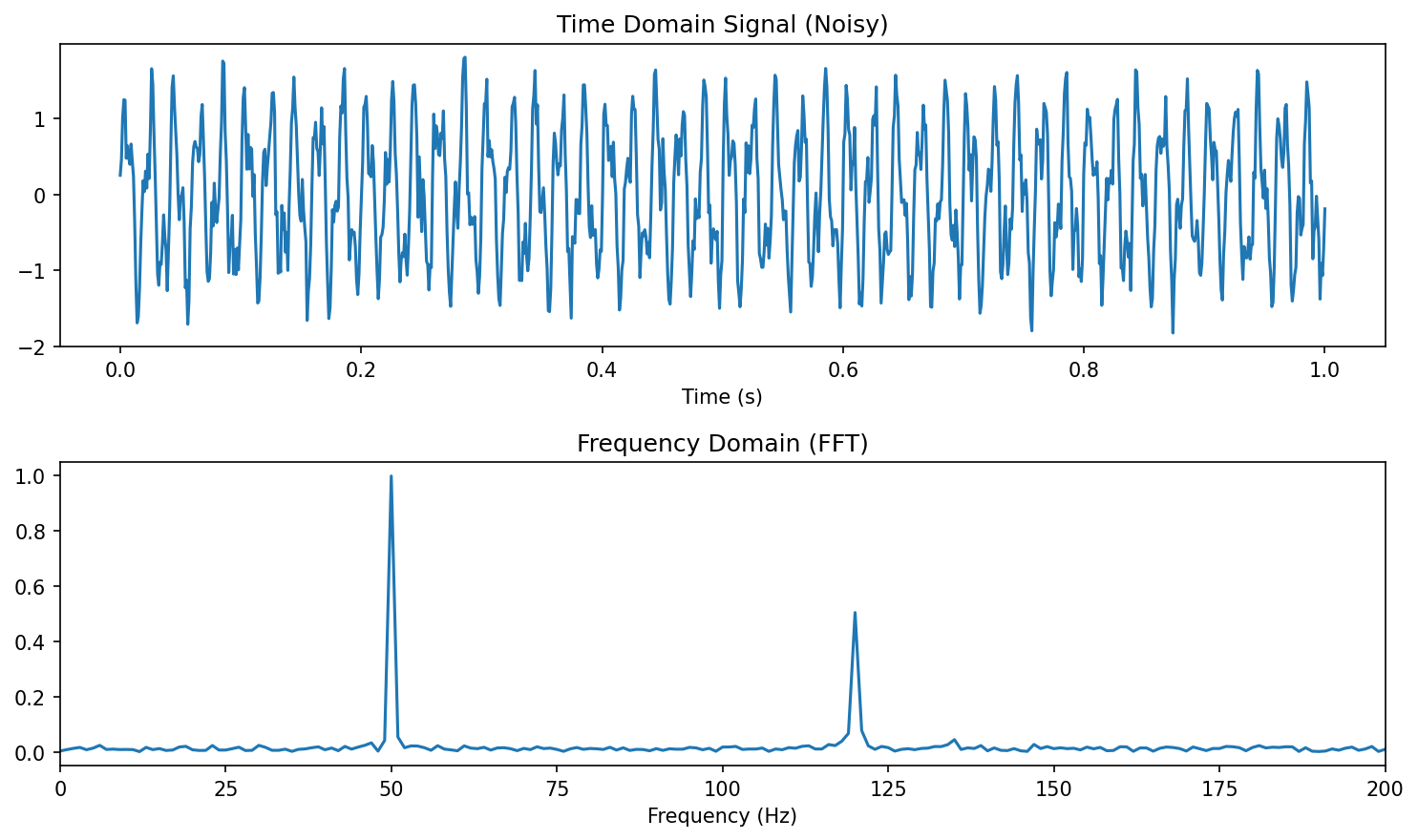
Diagnostic value. A specific \(\nu^*\) peak distinguishes “good” from “anomalous” motor cycles even when the time-domain signals look almost identical.

Sampling discipline. Recall Unit 2’s Nyquist–Shannon theorem: to detect frequency content up to \(\nu_{\max}\) you need a sampling rate of at least \(2\nu_{\max}\). Aliasing is the form of leakage that occurs during data acquisition and cannot be undone digitally.

Why complex-valued? The FFT has both magnitude and phase. The magnitude \(|\hat{x}|\) encodes “how much” of frequency \(\nu\); the phase encodes its alignment in time. For classification tasks the magnitude is usually enough; for reconstruction (e.g., ptychography in Unit 9) the phase is the entire game.

Common pitfalls. - Spectral leakage (window-induced): use a Hann or Hamming window before FFT. - DC dominance: subtract the mean before transforming, or its peak at \(\nu = 0\) swamps everything. - Wrong axis units: the frequency bin \(k\) corresponds to \(\nu_k = k / (N \Delta t)\). Get \(\Delta t\) right or your peaks land in the wrong place.

19. When the FFT Fails — Localised Signals

FFT assumes the signal is periodic over the whole window.

A transient — an acoustic-emission burst, a crack-initiation event, a single phonon pulse — is short in time but broad in frequency. The FFT finds its frequency content but cannot tell you when it happened.

The consequence

• Two signals with identical FFTs may differ in when the events occurred.
• For event detection / process monitoring (Unit 7) we need both axes.

Wavelet transform — the Ricker example Neuer, Michael et al., (2024), eq. 3.16: \[ \psi\!\left(\tfrac{t-b}{a}\right) \;\propto\; \frac{d^2}{dt^2}\, e^{-(t-b)^2 / a^2} \]

Continuous wavelet transform (CWT): \[ \mathrm{CWT}[x](a, b) \;=\; \frac{1}{\sqrt{|a|}} \!\int x(t)\, \psi\!\left(\tfrac{t-b}{a}\right) dt \]

Output is a function of width \(a\) (≈ inverse frequency) and position \(b\) (time) — a 2D time–frequency map.

Heisenberg-style trade-off. You cannot have arbitrarily high resolution in time and in frequency simultaneously. Wavelets parameterise the trade-off: narrow \(\psi\) → good time resolution, poor frequency resolution; wide \(\psi\) → the opposite.

Practical wavelet families. Ricker (mexican-hat) for symmetric transients; Morlet for oscillatory bursts; Haar for step changes. Choice is dictated by the physical event you hunt for. There is no “default” wavelet.

ML angle. A 1D CNN learns its own wavelet-like filters from data. Wavelets are the hand-engineered prior; CNNs are the data-driven version. Knowing the prior helps you interpret what the network learned.

20. Triggering — Cutting the Time Series

Many process signals are long, with short interesting windows:

• A rolling-mill cycle inside hours of idle.
• A laser pulse inside seconds of dwell.
• A loading cycle inside thousands of fatigue cycles.

Triggering extracts windows around events.

def trigger(x, threshold, window):
    return [x[i:i+window]
            for i in range(len(x)-window)
            if x[i] > threshold]

Why it matters

• Aligns repeated events for averaging.
• Reduces dataset size from gigabytes to megabytes.
• Lets you compare cycles directly — anomalies pop out as deviations from the mean cycle.

Connect: in Unit 7 (time-series ML) we will build models that learn the trigger criterion.

Threshold choice is domain-specific. A fatigue test triggers on load > 0.9 of peak; an acoustic-emission detector triggers on amplitude > 4× background RMS. The “right” threshold is whatever isolates the event of interest with high recall and tolerable false positive rate.

Triggering vs detection. Triggering uses a hand-set rule. Detection learns the rule. For known events with stable signatures, triggering wins on simplicity and robustness. For unknown or drifting events, learned detectors win on flexibility.

A subtle leakage trap. If the trigger is based on the target variable (e.g., trigger on “outcome > threshold”), you have effectively seen the label before training. Trigger must use only inputs available at run time.

21. Recap — the Transformation Toolbox

Goal	Tool	When
Centre at zero	mean subtraction	covariance, FFT phase
Bound to \([0,1]\)	min–max	image pixels, bounded sensors
Equalise spread	standardisation	kNN, PCA, regularised linear
Linearise multiplicative	log	power laws, dynamic range
Reveal change	derivative	baseline drift, anomaly
Reveal periodicity	FFT	stationary oscillations
Reveal localised periodicity	wavelet	transients, AE events
Isolate cycles	triggering	repetitive processes
Remove unit dependence	non-dimensionalisation	physics-aware ML

Rule of thumb: match the transform to what you want the model to see.

Use this slide as a reference card. Tell students the table is intended to live on the desk during their project work. Each row is “if your data has this property, try that tool.”

Multiple transforms compose. A typical stress–strain ML pipeline: shift to align elastic origins → standardise per channel → take first derivative → trigger on plastic onset → FFT to find Lüders-band frequency. Each transform is a modelling choice and each should be defensible.

No transformation is free. Every transform throws away information. Document them all. The same transform applied at training and inference time. In writing.

22. Pause & Reflect — Which Transform?

For each of the four signals below, which preprocessing would you apply first, and why?

(a) What would you apply first to a vibration spectrum from a rolling bearing, sampled at \(20\,\mathrm{kHz}\)?

Answer: FFT to find characteristic fault frequencies; subtract DC first.

(b) Grain-size measurements ranging from \(50\,\mathrm{nm}\) to \(50\,\mathrm{\mu m}\).

Answer: Log-transform to bring 3 decades onto a manageable scale.*

(c) Three sensors measuring temperature, pressure, current — fed into a kNN classifier.

Answer: Standardise so no single feature dominates the Euclidean distance.*

(d) Acoustic emission during fatigue — long quiet stretches, brief bursts.

Answer: Trigger on amplitude threshold; CWT inside each window for time–frequency content.*

Active learning checkpoint (~3 min). Run this as think-pair-share: 1. Think (60 s): each student picks an answer for one of the four signals. 2. Pair (90 s): turn to neighbour, compare and defend. 3. Share (60 s): cold-call two pairs, then reveal the recommended answer.

Calibration. Don’t reveal the answers as “the right one” — reveal them as “what most practitioners would default to, and why.” Push back if students suggest something unexpected and have a defence — there are often multiple valid answers (e.g., (b) could also be cube-root, depending on whether the underlying distribution is log-normal vs. gamma).

Time check. This is the natural place for a 3-minute mini-break — students refill coffee, you breathe.

§3 · Labels and Uncertainty

23. Labels Are the Hard Part

A supervised model is only as good as its labels.

In materials science, labels are:

• Sparse — few experiments, fewer per-pixel masks.
• Costly — domain expert time, \(\$\) per hour, hours per image.
• Subjective — expert interpretation drift over weeks of labelling.
• Often probabilistic — “phase A” is a continuum, not a Boolean.

Common scenarios

• TEM/SEM segmentation: hand-painted masks for grain boundaries, defects, particles.
• Phase classification: expert-assigned class from XRD or EBSD.
• Defect cataloguing: human review of thousands of optical images.

Note

Insight: the labelling process is itself a measurement chain (Unit 2) — with its own noise model.

Numbers to anchor. A trained TEM operator labels around 50 grain-boundary masks per hour; a state-of-the-art segmentation paper might use 500 such masks. That is a 10-hour investment per dataset before any modelling. This is why transfer learning (Unit 6) matters so much — it reuses upstream labels.

Frame labelling as a sensing problem. Every mask, every class assignment, is a measurement. Just as in Unit 2, there is signal (the true latent ground truth), noise (annotator disagreement), and bias (annotator-specific shortcuts). Treat labels with the same scepticism as raw sensor outputs.

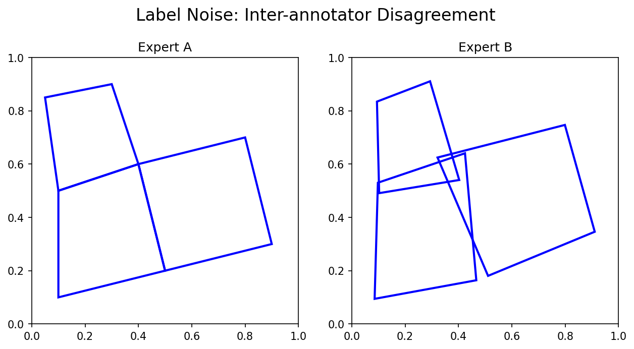
24. Inter-Annotator Variance

Two domain experts rarely agree pixel-for-pixel on:

• Grain boundary location (where exactly is the contrast threshold?).
• Phase mask boundary (gradual transitions).
• Particle vs. background near low-contrast edges.

Note

Quantify it! Compute Dice or IoU between annotators — this gives you the ceiling for any model’s performance when trained on either set of labels.

Two experts, same TEM micrograph, different masks. Their Dice agreement is 0.78 — no model trained on one expert’s labels can score above this against the other’s.

Bayesian view. A label is not the truth — it is a sample from \(p(\text{label} \mid \text{image, expert})\). The “true” mask is a latent variable. Modelling labels as point estimates throws away the disagreement information.

Practical strategy. When you have multiple annotators per image: 1. Compute inter-annotator agreement (Dice, IoU, Cohen’s kappa). 2. Use the consensus as supervision but report the agreement as the noise floor. 3. For ambiguous regions, train with probabilistic labels (next slide).

Common mistake. Reporting model accuracy of 0.95 when the inter-annotator Dice is 0.80 is suspicious — the model has likely learned annotator-specific quirks rather than the underlying physics. This is one of the easier silent failures to catch if you measure inter-annotator variance up front.

25. Probabilistic Labels and Softmax

Hard label — one-hot vector \(\mathbf{y} = [0, 1, 0]\).

Soft label — distribution \(\mathbf{y} = [0.1, 0.7, 0.2]\).

For a classifier producing logits \(z_\ell\), the softmax converts them to probabilities: \[ p(\ell \mid \mathbf{x}) \;=\; \frac{e^{z_\ell(\mathbf{x})}}{\sum_{\ell'} e^{z_{\ell'}(\mathbf{x})}} \]

The output sums to 1 — interpret as a probability over classes.

Why it matters in materials science

• A “phase A” label may really mean 80% A, 20% A+B at a phase boundary.
• Probabilistic labels propagate the labeller’s uncertainty into training.
• Softmax outputs let you threshold — flag \(\max_\ell p_\ell < 0.6\) for human review.

Connect: Unit 12 (Gaussian processes, uncertainty-aware regression) treats this principle in full generality.

Calibration. A model can be highly accurate yet poorly calibrated — confidently wrong. Rule of thumb: a well-calibrated 80%-confident prediction is right 80% of the time. Reliability diagrams are the diagnostic. Temperature scaling (a single learned scalar that divides the logits) is the cheapest fix.

Softmax temperature. Dividing logits by \(T\) before softmax makes the distribution sharper (\(T < 1\)) or flatter (\(T > 1\)). \(T = 1\) at training; lowering it at inference gives sharper predictions (and worse calibration). It’s a knob, not a fix.

26. Bayesian View of Models — Prior, Likelihood, Posterior

Bayes’ rule McClarren, Ryan G., (2021):

\[ \underbrace{p(\mathbf{w} \mid \mathcal{D})}_{\text{posterior}} \;=\; \frac{ \overbrace{p(\mathcal{D} \mid \mathbf{w})}^{\text{likelihood}} \; \overbrace{p(\mathbf{w})}^{\text{prior}} }{ \underbrace{p(\mathcal{D})}_{\text{evidence}} } \]

Reading it

• Prior: what you believe about parameters \(\mathbf{w}\) before seeing data.
• Likelihood: how plausible the data is for given \(\mathbf{w}\).
• Posterior: updated belief after seeing data.

Why this matters today

• Standard ML returns a point estimate (one \(\mathbf{w}^*\) that maximises the likelihood).
• A Bayesian treatment returns a distribution over \(\mathbf{w}\) → uncertainty on every prediction.
• Regularization (next section) is exactly a prior on \(\mathbf{w}\):
  • L2 penalty \(\lambda \|\mathbf{w}\|_2^2\) ↔︎ Gaussian prior.
  • L1 penalty \(\lambda \|\mathbf{w}\|_1\) ↔︎ Laplace prior.

Connect: Unit 12 (GPs) takes the Bayesian view all the way; today we just need its vocabulary.

Why introduce Bayes here. Two reasons. First, it gives a clean explanation of why regularization works (it is a prior, not a hack). Second, it is the formal framework for expressing uncertainty in predictions — which we need for soft labels above and for GP regression in Unit 12.

MAP vs MLE. Maximum likelihood (MLE) returns the \(\mathbf{w}\) that fits training data best — overfits without regularization. Maximum a posteriori (MAP) returns the \(\mathbf{w}\) that maximises the posterior — equivalent to MLE with a regularization term.

Computational cost. Full posteriors are intractable for any non-toy model. MCMC (Metropolis–Hastings) and variational inference are the workhorses. For some problems the posterior is closed-form (conjugate priors, GPs); we use those when we can.

§4 · Bias, Variance, and Parsimony

27. Underfit, Good Fit, Overfit

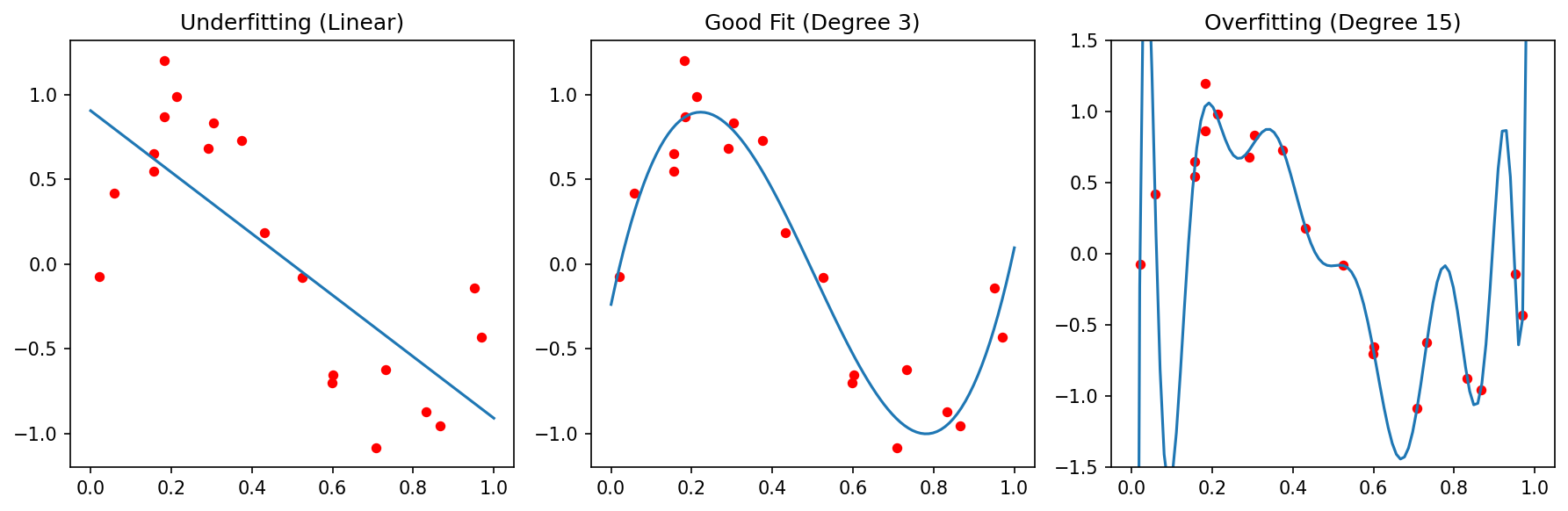
Three fits to the same data: too stiff (underfit, high bias), well-balanced, too flexible (overfit, high variance). Adapted from Sandfeld, Stefan et al., (2024).

Anchor in concrete numbers. Sandfeld’s quadratic example: balanced fit gives \(\mathrm{MSE}_{\text{train}} = 1.1, \mathrm{MSE}_{\text{test}} = 2.7\) (close — good generalisation). Degree-13 polynomial gives \(\mathrm{MSE}_{\text{train}} = 0.1, \mathrm{MSE}_{\text{test}} = 7098\) — five orders of magnitude. The training error tells you nothing about test performance for an over-flexible model.

Diagnostic on the chalkboard. Plot training and test error as a function of model complexity. Training error monotonically decreases. Test error has a U-shape: high at both extremes, minimum in the middle. The minimum is the model you want.

Materials caveat. Many materials datasets are small (\(N < 100\)). The test-error U is noisy. Trust the U-shape qualitatively, not its exact minimum location.

28. The Bias–Variance Decomposition

For squared-error loss Sandfeld, Stefan et al., (2024), eq. after MSE:

\[ \mathbb{E}\bigl[(\hat{y} - y)^2\bigr] \;=\; \underbrace{\bigl(\mathbb{E}\hat{y} - y\bigr)^2}_{\mathrm{Bias}^2} \;+\; \underbrace{\mathrm{Var}(\hat{y})}_{\text{Variance}} \;+\; \underbrace{\sigma^2}_{\text{Noise}} \]

• Bias: systematic error of an averaged prediction.
• Variance: sensitivity of the prediction to a particular training set.
• Noise: irreducible — the floor set by the data.

Practical reading

• Underfit → high bias, low variance. Cure: more flexible model, more features.
• Overfit → low bias, high variance. Cure: more data, fewer parameters, regularization.
• Good fit → bias and variance both small relative to the noise floor.

Materials reality: \(\sigma^2\) is often large (small samples, expensive measurements). Don’t chase a model below the noise.

Tie back to Unit 2. The noise term \(\sigma^2\) is exactly the aleatory uncertainty introduced in Unit 2 — irreducible, set by physics and detector electronics. The bias and variance are epistemic — reducible with better models or more data.

The wrong mental model. Students often think “more data always helps.” It helps with variance. It does not help with bias. A linear model on intrinsically nonlinear data will not improve no matter how many points you add.

Materials engineering analogy. Bias is like a systematic calibration offset on a load cell — repeating the experiment many times doesn’t fix it. Variance is like measurement noise — averaging many trials does fix it.

29. Parsimony — Occam’s Razor

Entia non sunt multiplicanda praeter necessitatem.

“Entities should not be multiplied beyond necessity.” — William of Ockham, 14th c.

McClarren’s example McClarren, Ryan G., (2021):

• True relationship: \(y = 3x_1 + \delta\), with \(\delta \sim \mathcal{N}(0, \sigma^2)\).
• Available features: \(x_1, \dots, x_{50}\) (\(x_{2..50}\) are pure noise).
• Fit a 50-parameter linear model → zero training error.
• Test error → catastrophic. The 49 spurious coefficients have memorised noise.

The lesson

A model with capacity \(\geq\) dataset size can memorise noise. Adding the right kind of bias toward simplicity is the only protection.

Practical consequences

• Prefer linear/quadratic over high-degree polynomials.
• Prefer fewer hidden layers, fewer features.
• Add an explicit parsimony term to the loss → regularization.

Quantify the trap. McClarren’s setup is a clean failure: only \(x_1\) is signal; the linear model’s 50 parameters are enough degrees of freedom to fit any 50 points. The training \(R^2 = 1\). This is exactly the situation where a single number (\(R^2\)) tells you nothing useful and you need held-out validation.

Common materials-data analogue. A small DOE (\(N = 30\)) with many candidate features (processing temperature, pressure, time, and 47 derived ratios). Fit a regression with all features and “discover” highly significant coefficients on noise.

Sanity check. Compute training error and a permutation test: shuffle \(y\), refit. If the model still achieves low training error, the model class is too flexible for the data.

30. Regularization — Parsimony in the Loss

Augment the loss: \[ \mathcal{L}_{\text{reg}}(\mathbf{w}) \;=\; \mathcal{L}_{\text{data}}(\mathbf{w}) \;+\; \lambda\, \Omega(\mathbf{w}) \]

Two canonical penalties

• L2 / Ridge: \(\Omega(\mathbf{w}) = \|\mathbf{w}\|_2^2 = \sum_j w_j^2\). Shrinks all weights toward zero; keeps them all non-zero.
• L1 / Lasso: \(\Omega(\mathbf{w}) = \|\mathbf{w}\|_1 = \sum_j |w_j|\). Drives many weights exactly to zero — feature selection built in.

Bayesian re-reading

• L2 ↔︎ Gaussian prior \(\mathbf{w} \sim \mathcal{N}(0, \sigma_w^2 \mathbf{I})\).
• L1 ↔︎ Laplace prior \(\mathbf{w} \sim \mathrm{Laplace}(0, b)\).
• \(\lambda\) ↔︎ inverse prior strength.

Materials value. Lasso applied to McClarren’s example zeros out 49 noise features, recovers \(w_1 \approx 3\). The model literally tells you which features matter.

Choosing \(\lambda\). Cross-validation. Sweep \(\lambda\) over a logarithmic grid; pick the value with lowest CV error. We will see this concretely in §5.

Why both Ridge and Lasso exist. Ridge handles correlated features gracefully — it spreads weight across them. Lasso picks one and zeros the rest, which is sharper but less stable when features are nearly collinear. Elastic net combines both penalties.

Connect forward. When we discuss neural networks, weight decay = L2 regularization on the network weights. Dropout, batch norm, early stopping are all forms of regularization. The whole field of deep learning is the search for implicit regularizers that work in high dimensions.

§5 · Robust Validation

31. The Holdout — Train/Test Split

The simplest validation strategy Sandfeld, Stefan et al., (2024):

1. Randomly split data: 70–80% train, 20–30% test.
2. Fit on train.
3. Evaluate on test → estimate of generalisation.

Quick, cheap, often used.

from sklearn.model_selection import train_test_split
X_tr, X_te, y_tr, y_te = train_test_split(
    X, y, test_size=0.2, random_state=42)

The risks

• For small datasets (typical in materials), the split is random — a single unlucky split can mis-estimate performance by 50%.
• All data points contribute equally to a single error estimate; no measure of variance.
• Selection bias: if rare classes end up entirely in train or test, you don’t notice.

Sandfeld’s experiment: 100 random 60/40 splits on the same data → 100 different MSEs, sometimes off by 5×. The holdout gives you one of those 100 numbers.

Set the random seed. For reproducibility, but understand that the seed is a choice. Reporting “test error 0.07” without saying which seed is meaningless on small datasets. Good practice: report mean ± std across many seeds.

The 80/20 ratio is folklore. It comes from the Pareto distribution rule of thumb, not from any theorem. For very small datasets (N < 50) you may want larger train fractions (90/10) or you may want to abandon holdout entirely (next slides).

The validation/test distinction. If you only train one model with one set of hyperparameters, “test” and “validation” mean the same thing. As soon as you tune hyperparameters on the held-out set, you need three sets — train (fit), validation (tune), test (final report). Conflating validation and test is the most common cause of optimistic generalisation estimates in published papers.

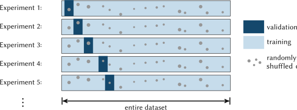
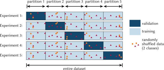
32. K-Fold Cross-Validation

The recipe Sandfeld, Stefan et al., (2024):

1. Split data into \(k\) equal folds at random.
2. For \(i = 1 \ldots k\):
   • Train on the \(k-1\) folds excluding \(i\).
   • Test on fold \(i\), record \(\mathrm{MSE}_i\).
3. Report \[ \overline{\mathrm{MSE}} \;=\; \frac{1}{k}\sum_{i=1}^{k} \mathrm{MSE}_i \quad\text{and}\quad \mathrm{std}(\mathrm{MSE}_i). \]

Why it’s better than holdout

• Every point is used for both training and testing — no waste.
• The std across folds tells you how stable the estimate is.
• Less sensitive to a single unlucky split.

Cost

• \(k\) trainings instead of 1. For deep nets, often \(k = 3\) or \(5\), not \(10\).

Defaults

• \(k = 10\) for moderate datasets (\(N \sim 10^3\)).
• \(k = 5\) for compute-bound situations.
• \(k = 3\) when even that is too expensive.

Variance of the estimator. \(\overline{\mathrm{MSE}}\) has less variance than a single holdout because it averages \(k\) estimates. Use the across-fold std as an informal error bar — it is biased, but useful as a “is the model stable?” indicator.

A subtlety. The k-fold estimate is a biased estimate of the generalisation error, because each model is trained on \((k-1)/k\) of the data, not all of it. The bias goes to zero as \(k \to N\) (LOOCV).

Compute discipline. For deep learning, k-fold is often skipped because \(k\) trainings × hours each is impractical. The honest replacement is bootstrapped confidence intervals on a single holdout, or holdout × multiple seeds.

33. Leave-One-Out (LOOCV) and Stratified Folds

LOOCV — \(k = N\).

• Each fold is a single point.
• \(N\) trainings — usually impractical above \(N \sim 10^3\).
• Lowest possible bias for a CV estimator.
• Very useful for very small datasets (\(N < 30\), common in materials).

LOOCV

Stratified k-fold

• Each fold preserves the class distribution of the whole dataset.
• Critical for imbalanced problems: rare-defect detection, minority-phase identification.
• sklearn.model_selection.StratifiedKFold.

Stratified k-fold

When to stratify on a continuous target. Bin the target into a few quantile buckets and stratify on the bucket. Prevents folds where one chunk of the target distribution is absent.

Multi-label stratification. When a sample has multiple labels (e.g., contains both phase A and phase B), naive stratification fails. Use IterativeStratification from the scikit-multilearn library, or accept a small imbalance.

Leakage warning (preview). Stratifying by a feature that encodes the target (e.g., specimen ID where each ID has only one class) is fine. Stratifying by something that is the target leaks. Be precise about what you stratify on.

34. Data Leakage — the Silent Killer

Definition. Information from the test set influences the training process — directly or indirectly. The reported performance is then optimistic by an unknown amount.

Symptoms

• Cross-validation score >> realistic deployment score.
• Performance drops sharply on a “true” external dataset.
• Even simple models match deep nets — both are exploiting the leak.

Cause: a discipline failure, not a bug. Almost all real cases come from one of three patterns on the next slides.

Three classes you must know

1. Pre-processing leakage — fitting transforms on train+test combined.

2. Temporal leakage — using future to predict past.

3. Group / spatial leakage — same physical entity in train and test.

The general framing. Treat the test set as if it were data you will only see in production. Anything you do during training that uses test-set values is a leak. This includes: scaling, imputation, feature selection, hyperparameter tuning.

War story. A widely cited 2019 paper on superconductor Tc prediction was found to have group-leakage: the same compound family appeared in train and test under different synthesis conditions. The 0.95 R² collapsed to 0.6 on a clean re-evaluation. The model was fine. The validation was broken.

35. Pre-Processing Leakage

The wrong way:

X_scaled = StandardScaler().fit_transform(X)
X_tr, X_te, y_tr, y_te = train_test_split(X_scaled, y)
model.fit(X_tr, y_tr)

The scaler computed \(\mu, \sigma\) on \(X\) — including the test rows. Test-set statistics leaked into training.

The right way:

X_tr, X_te, y_tr, y_te = train_test_split(X, y)
scaler = StandardScaler().fit(X_tr)   # train only
X_tr = scaler.transform(X_tr)
X_te = scaler.transform(X_te)
model.fit(X_tr, y_tr)

scikit-learn’s Pipeline does this for you:

Pipeline([("scale", StandardScaler()),
          ("model", Lasso())])

Subtle but ubiquitous. Almost every student does this once. The damage is usually small (mean and std are stable for large \(N\)) but invisible. For small \(N\) or strong outliers it can matter a lot.

Operations that leak when fitted on full data. - Standardisation, min–max scaling. - Imputation of missing values (using full-data means). - Feature selection (e.g., picking top-\(k\) features by correlation with \(y\)). - PCA fitted on full data.

The Pipeline pattern. sklearn.pipeline.Pipeline makes the right thing the default. Inside cross-validation, the pipeline is refit on every training fold, automatically.

36. Temporal Leakage

Time has a direction. You cannot use \(x(t+\Delta t)\) to predict \(y(t)\).

The wrong way: randomly shuffle a time series and split. The resulting training set has data points that come after test-set points — a model can exploit short-range temporal autocorrelation that won’t be there at deployment.

The right way: time-aware split.

─────train─────┃────val───┃───test───→ time
               t1         t2          T

• Train: \(t < t_1\).
• Validation: \(t_1 \le t < t_2\).
• Test: \(t \ge t_2\).

Walk-forward (rolling) CV for time series:

• Fold \(k\): train on \([0, T_k)\), test on \([T_k, T_k + \Delta T)\).
• Increment \(T_k\), repeat.
• Honestly simulates “predict next month from past data.”

Materials examples

• Process monitoring (Unit 7) — predict tomorrow’s drift from yesterday’s logs.
• Operando spectroscopy — predict reaction rate at \(t+\Delta t\) from spectrum at \(t\).

sklearn.model_selection.TimeSeriesSplit.

Subtle temporal leaks. - Rolling features. If a “30-day moving average” feature includes test-period data, that is leakage even with a time-aware split. - Future-aware target encoding. Encoding categorical variables by their mean target over all time leaks future information into the encoding. - Hyperparameter tuning. Tuning on a random k-fold of a time series leaks just as badly as random train/test.

Connect forward. Unit 7 spends most of its time on this — recurrent and Transformer architectures, attention masks, walk-forward validation as the only honest CV.

37. Group / Spatial Leakage

The trap. Multiple data points share an underlying physical entity:

• Several TEM micrographs of the same specimen.
• Several stress-strain curves from the same fatigue coupon.
• Several DFT calculations on the same compound family.

If random splitting puts some of those rows in train and others in test, the model can recognise the entity rather than the property.

The cure: group-based splitting.

from sklearn.model_selection import GroupKFold
gkf = GroupKFold(n_splits=5)
for tr, te in gkf.split(X, y, groups=specimen_id):
    model.fit(X[tr], y[tr])
    score = model.evaluate(X[te], y[te])

The split now respects the physical grouping — the entire specimen is in either train or test, never both.

Note

Materials default: if there is a specimen_id column, your default CV is GroupKFold.

Why it bites in materials science. Specimens are expensive — you take many measurements per specimen. The variance within a specimen is small (same processing, same composition, same defects); the variance across specimens is large (different batches, operators, environments). Random splitting tests interpolation within specimens — trivial. Group splitting tests generalisation across specimens — what you actually want.

Detection heuristic. If your random-CV score is much higher than your group-CV score, you have group structure that random CV is exploiting. The gap is a useful diagnostic.

Connect forward. Unit 6 (transfer learning) takes group leakage to its extreme — “how well does a model trained on alloy family A generalise to alloy family B?” The answer is “less well than you think,” and group-CV is what tells you so.

38. Pause & Reflect — Spot the Leak

For each scenario, identify the leakage — and the fix.

(a) You scale all features with StandardScaler.fit_transform(X) and then split into train/test.

Pre-processing leak. Fix: fit scaler on train only.

(b) You split a year of process data 80/20 at random and report 0.95 \(R^2\).

Temporal leak. Fix: train on first 80%, test on last 20% chronologically.

(c) You collected 20 micrographs from each of 5 fatigue specimens. Random 5-fold CV gives Dice 0.92; on a 6th specimen, Dice = 0.55.

Group leak. Fix: GroupKFold on specimen_id.

(d) You select the top-50 most correlated features with \(y\) on the full dataset, then run k-fold CV.

Pre-processing leak via feature selection. Fix: feature selection inside each fold.

Active learning checkpoint (~3 min). Same think-pair-share format as slide 22. Cold-call two pairs, then reveal answers.

Why this works as a teaching device. Each scenario is a real and common mistake — students may be making one of them right now in their thesis project. The discomfort of recognition is exactly the learning signal.

The taxonomy is the punchline. All four collapse to “test data influenced training.” That single sentence is the core of §5.

§6 · Error Measures

39. Why Error Measures Matter

A loss function trains the model. A metric reports performance. They need not be the same.

• Train with MSE because it’s smooth (gradient-friendly).
• Report MAE because it’s interpretable (in the same units as the target).
• Track \(R^2\) because it’s scale-free and lets you compare across datasets.

A metric encodes a value judgment.

• \(\mathrm{MAE}\) treats all errors linearly.
• \(\mathrm{MSE}\) punishes large errors disproportionately.
• \(\mathrm{Recall}\) favours catching positives over avoiding false alarms.

Different problems demand different metrics:

• Regression — MAE, MSE, RMSE, \(R^2\), MSLE.
• Classification — accuracy, precision, recall, F1, ROC-AUC.
• Segmentation — IoU, Dice.

Note

Pick the metric that matches what you actually care about. Defects you must catch → recall. Calibrated property predictions → MSE / \(R^2\). Sample size where outliers dominate → MAE.

The cardinal sin. Reporting accuracy on an imbalanced classification problem (“99% accuracy at detecting cracks!” when only 1% of samples have cracks — a model that always predicts “no crack” achieves 99%). Materials datasets are often imbalanced. Default to precision / recall / F1, not accuracy.

Multiple metrics. Always report at least one primary metric (the one tied to the business objective) and one interpretable metric (so a domain expert can sanity-check). For dislocation segmentation: primary = IoU, interpretable = “fraction of dislocation length recovered.”

40. Regression Metrics — MAE, MSE, RMSE

\[ \mathrm{MAE} = \frac{1}{n}\sum_{i=1}^n |y_i - \hat{y}_i| \] \[ \mathrm{MSE} = \frac{1}{n}\sum_{i=1}^n (y_i - \hat{y}_i)^2 \] \[ \mathrm{RMSE} = \sqrt{\mathrm{MSE}} \]

Properties

• \(\mathrm{MAE}, \mathrm{RMSE}\) in the units of \(y\) — directly interpretable.
• \(\mathrm{MSE}\) in squared units — opaque but smooth.
• \(\mathrm{MAE} \le \mathrm{RMSE}\) always; equality iff all errors are equal.

Outlier sensitivity

• MSE is dominated by the largest residual (squares it).
• MAE is robust — a single huge error contributes linearly.

Pick MSE when

• Large errors must be strongly penalised (safety-critical predictions).
• Smooth gradient is needed (training).

Pick MAE when

• Outliers are present and cannot be cleaned.
• The cost of an error grows linearly with its size (most engineering settings).

Decomposition. \(\mathrm{MSE} = \mathrm{Bias}^2 + \mathrm{Variance}\). Useful when diagnosing models — high MSE with low bias means high variance (overfitting); high MSE with low variance means high bias (underfitting). Connect back to slide 28.

MSLE preview. When the target spans orders of magnitude (grain size, fatigue life), RMSE is dominated by the largest values. The mean-squared-log error \(\mathrm{MSLE} = \frac{1}{n}\sum (\log(y_i) - \log(\hat{y}_i))^2\) is a relative metric — better suited.

41. The \(R^2\) Coefficient

\[ R^2 \;=\; 1 - \frac{\sum_i (y_i - \hat{y}_i)^2}{\sum_i (y_i - \bar{y})^2} \;=\; 1 - \frac{\mathrm{MSE}_{\text{model}}}{\mathrm{MSE}_{\text{baseline}}} \]

Interpretation: “fraction of variance in \(y\) explained by the model.”

• \(R^2 = 1\) → perfect fit.
• \(R^2 = 0\) → the model is no better than predicting \(\bar{y}\).
• \(R^2 < 0\) → the model is worse than the constant-mean baseline.
• Scale-invariant: comparable across datasets and units.

Caution: \(R^2\) alone is not enough McClarren, Ryan G., (2021).

• A high \(R^2\) does not imply a useful model. (McClarren’s overfit example: training \(R^2 = 1\), useless predictions.)
• Always report \(R^2\) on held-out data, not training.
• Pair \(R^2\) with a physical metric (RMSE in units, residual plots).

Adjusted \(R^2\). Penalises additional features that don’t help — \(R^2_{\text{adj}} = 1 - (1 - R^2)\frac{n-1}{n-p-1}\) where \(p\) is the number of features. Ordinary \(R^2\) rises monotonically with \(p\) on training data; adjusted does not.

Negative \(R^2\) is real. A model that systematically predicts the wrong sign on the test set has \(R^2 < 0\). Reporting “\(R^2 = -0.3\)” is bad news but it’s honest — the model is worse than the constant mean.

Residual plots. Plot \(\hat{y}_i - y_i\) against \(\hat{y}_i\). Random scatter → good. Trend → systematic bias. Funnel shape → variance scales with magnitude (consider log transform on \(y\)).

42. Confusion Matrix — the Atom of Classification

For a binary problem (“defective” = 1):

	Pred 0 (no defect)	Pred 1 (defect)
True 0	TN	FP (Type I)
True 1	FN (Type II)	TP

\[ \mathrm{Accuracy} = \frac{\mathrm{TP} + \mathrm{TN}}{\mathrm{TP} + \mathrm{TN} + \mathrm{FP} + \mathrm{FN}} \]

Sandfeld, Stefan et al., (2024)

The cost is asymmetric.

• Missing a defect (FN) → unsafe part ships → expensive recall, lawsuits.
• Calling a good part bad (FP) → unnecessary scrap → expensive but contained.

A balanced metric like accuracy hides this asymmetry. Precision and recall reveal it.

For multi-class: confusion matrix is \(K \times K\). Off-diagonal = misclassifications. Heat-map it.

Imbalance is the rule, not the exception. Defect detection: 1% defects → 99% accuracy by predicting “no defect” always. Phase identification: minority phases buried in majority. Always report the confusion matrix, not just accuracy.

Decision threshold matters. A binary classifier outputs a probability; the threshold 0.5 is a default, not a law. Adjusting the threshold trades precision for recall — the ROC and PR curves visualise this trade-off across thresholds.

Multiclass extensions. “Macro-averaged precision” treats each class equally; “weighted” weights by class frequency; “micro” pools all decisions. Pick one and say which one in the methods section.

43. Precision and Recall

\[ \mathrm{Precision} = \frac{\mathrm{TP}}{\mathrm{TP} + \mathrm{FP}} \] of what I called positive, how much actually was?

\[ \mathrm{Recall} = \frac{\mathrm{TP}}{\mathrm{TP} + \mathrm{FN}} \] of what was actually positive, how much did I find?

Synonyms

• Recall = Sensitivity = True positive rate.
• Precision = Positive predictive value.

They trade off. Lower the decision threshold → recall ↑, precision ↓.

Pick by use case

• Cancer screening → recall (don’t miss any).
• Spam filter → precision (don’t trash real mail).
• Defect inspection → recall (every miss is a field failure).
• Search ranking → precision (top results matter most).

Materials examples

• Defect detection in SEM: recall first.
• Phase classification of a known mixture: precision and recall both matter → use F1.

Operating point. A real model is deployed at one threshold. Pick it from the PR curve to match the cost ratio of FN to FP. If a missed defect costs 100× a false alarm, operate where \(\partial\mathrm{Recall}/\partial\mathrm{Precision} \approx 100\).

Average precision. The area under the PR curve summarises performance across all thresholds. More informative than accuracy on imbalanced problems; preferred for ranked-retrieval tasks.

Don’t confuse with confidence. A model can have high precision and recall but be poorly calibrated — confidence values that don’t match true probabilities. Calibration is a separate concern (slide 25).

44. F1 / Dice Coefficient

\[ \mathrm{F1} \;=\; \frac{2\,\mathrm{Precision}\cdot\mathrm{Recall}}{\mathrm{Precision} + \mathrm{Recall}} \;=\; \frac{2\,\mathrm{TP}}{2\,\mathrm{TP} + \mathrm{FP} + \mathrm{FN}} \]

The harmonic mean of precision and recall — close to the minimum of the two, so a model with one near-zero score is heavily punished.

In segmentation, the same quantity is called the Dice coefficient.

Sandfeld, Stefan et al., (2024)

Dice for segmentation

For predicted region \(A\) and true region \(B\): \[ \mathrm{Dice}(A, B) \;=\; \frac{2|A \cap B|}{|A| + |B|} \]

• \(\mathrm{Dice} = 1\) → perfect overlap.
• \(\mathrm{Dice} = 0\) → no overlap.

Single-metric trap. A high Dice can hide systematic over- or under-segmentation. Always pair with precision and recall to know which way the model fails.

Why harmonic mean. The arithmetic mean of (precision = 1, recall = 0) is 0.5 — looks fine but the model is useless. The harmonic mean is 0 — correctly flags the failure.

\(F_\beta\). Generalises F1: \(F_\beta = (1+\beta^2) \frac{P\,R}{\beta^2 P + R}\). \(\beta = 1\) treats precision and recall equally; \(\beta > 1\) favours recall; \(\beta < 1\) favours precision. Useful when the asymmetric cost is known.

Per-class vs averaged. For multiclass segmentation, report Dice per class and a macro-average. A single overall number hides minority-class collapse.

45. IoU / Jaccard — the Other Overlap Metric

\[ \mathrm{IoU}(A, B) \;=\; \frac{|A \cap B|}{|A \cup B|} \;=\; \frac{\mathrm{TP}}{\mathrm{TP} + \mathrm{FP} + \mathrm{FN}} \]

Relation to Dice: \[ \mathrm{Dice} = \frac{2\,\mathrm{IoU}}{1 + \mathrm{IoU}} \]

Both range \([0, 1]\). IoU is always smaller than (or equal to) Dice for the same prediction.

When IoU is the convention

• Object detection (mean Average Precision at IoU thresholds 0.5, 0.75).
• Instance segmentation in computer vision benchmarks.
• Materials microscopy benchmarks (defect / particle / grain segmentation).

When Dice is the convention

• Medical image segmentation.
• Many materials-segmentation papers (especially TEM).

Either is fine — but be explicit.

Sandfeld’s TEM example summary Sandfeld, Stefan et al., (2024), Table 11.2:

Mask	IoU	Dice	Precision	Recall
A (under-prediction)	0.68	0.81	1.00	0.68
B (over-prediction)	0.88	0.94	0.88	1.00
C (mixed errors)	0.67	0.80	0.85	0.75

Mask A has perfect precision — every predicted pixel is dislocation — but only 0.68 recall. Mask B has perfect recall — every dislocation pixel is found — but precision 0.88 because of false positives. Mask C is the worst overall, even though its IoU and Dice are similar to mask A. The lesson: a single number cannot diagnose the failure mode. Always report at least precision and recall alongside IoU/Dice.

46. Categorical Cross-Entropy — the Default Multiclass Loss

For \(K\) classes with one-hot true label \(\mathbf{y}\) and predicted probabilities \(\hat{\mathbf{p}} = \mathrm{softmax}(\mathbf{z})\) Sandfeld, Stefan et al., (2024), eq. 11.20:

\[ \mathcal{L}_{\mathrm{CE}} \;=\; -\sum_{k=1}^{K} y_k \log \hat{p}_k \]

For binary: \[ \mathcal{L} = -[y\log \hat{p} + (1-y)\log(1-\hat{p})] \]

Punishes confident wrong predictions disproportionately — \(\log(0)\) blows up.

Why cross-entropy is the standard loss

• It’s the negative log-likelihood under a categorical distribution → maximum-likelihood interpretation.
• Smooth and convex in the logits — gradient-friendly.
• Recovers the right calibrated probabilities (when the model has the capacity).

Connect: later units use cross-entropy to train CNNs (Unit 5), language-model heads, and even contrastive losses.

Numerical stability. Computing \(\log(\mathrm{softmax}(z))\) naively underflows for large \(|z|\). Frameworks provide a fused log_softmax and nll_loss, or CrossEntropyLoss directly on logits. Always feed logits, not softmaxed probabilities.

Label smoothing. Replace one-hot \(\mathbf{y}\) with \((1 - \alpha)\mathbf{y} + \alpha/K\) to discourage extreme overconfidence. Improves calibration; small accuracy cost.

Class-weighted CE. For imbalanced problems, weight each class inversely to its frequency. The cheap, correct fix for “my model always predicts the majority class.”

§7 · Wrap-Up

47. Putting It Together — a Materials ML Recipe

1. Inspect. df.describe(), plot histograms and scatter, check dtypes, sample IDs, units.

2. Clean. Handle NaNs by source-fix → mark → interpolate → drop, in that order. Identify outliers; decide artifact vs rare event with a domain expert in the room.

3. Transform. Pick a transform per physical reasoning, not by reflex. Standardise after splitting. Document every transform.

4. Validate. Choose CV that matches the data: GroupKFold for grouped data, TimeSeriesSplit for temporal data, StratifiedKFold for imbalanced classes. Never random k-fold without verifying group structure.

5. Measure. Pick a metric that reflects the cost of errors in the application. Report the confusion matrix, not just accuracy.

6. Diagnose. Compare CV variance to mean. Compare random-CV vs group-CV. Check residual plots. Permute labels — does the model still “succeed”?

Use this slide as a closing mnemonic. Inspect, Clean, Transform, Validate, Measure, Diagnose. If a student remembers nothing else from today, this six-step checklist is the working recipe.

Iterate. It is a loop, not a sequence. Issues found in step 6 send you back to step 2 or 3. The number of iterations is a useful proxy for project maturity.

48. Things Most Teams Get Wrong

The greatest hits of materials-ML failures:

• Scaling on full data → leakage.

• Random k-fold on grouped data → over-optimistic scores.

• Reporting accuracy on imbalanced problem → meaningless.

• Ignoring inter-annotator variance → modelling noise.

• Single-number metric on segmentation → hides failure mode.

• Random shuffle on time series → temporal leakage.

• Outliers removed by 3σ rule without physics check → losing rare events.

• High \(R^2\) on training → no statement about generalisation.

• Tuning hyperparameters on the test set → leakage by another name.

• “It works on my data” without cross-instrument validation → distribution shift in disguise.

Use this slide as a checklist. Tell students they will revisit it before each project milestone. Have they done any of these? If yes, fix before reporting results.

Connect to the literature. Each item maps to a common pattern of erratum / retraction in published materials-ML work. Cite a couple if time permits — students remember cautionary tales better than abstract rules.

49. Looking Ahead — Unit 4

Unit 4: From classical microstructure metrics to learned representations.

• Inputs: segmented images, point sets, crystallographic data — all preprocessed with today’s tools.
• Goal: turn microstructures into vectors a model can consume.
• Methods: texture descriptors, two-point statistics, eigen-microstructures (PCA on standardised images!), latent-space encoders.

Today’s tools you’ll need next week

• Standardisation → eigen-microstructures need it.
• Group-based CV → samples come from the same alloy.
• IoU/Dice → for segmentation labels feeding into representations.
• Bayesian view → priors on latent codes.

Make the bridge concrete. Show one slide preview of an eigen-microstructure (will be in next week’s deck). Explain that PCA without standardisation gives PC1 = “which image is the brightest” — totally useless. Standardisation is what makes PCA find physically meaningful modes of variation.

Reading bridge. The Sandfeld §11.5 chapter you skimmed today is the prerequisite for the §15 PCA chapter you’ll need next week. Save the time investment by reading the preprocessing chapter properly now.

50. Reading & Exercises

Required reading

• Sandfeld, Materials Data Science, §11.5, §11.7, §11.8, §16.2.
• Neuer, Machine Learning for Engineers, Ch. 3.
• McClarren, Machine Learning for Engineers, Ch. 1 (especially §1.5 Cross-Validation).

Optional

• Bishop, PRML, §1.3 (model selection), §1.5 (decision theory).
• Murphy, MLAPP, Ch. 1 (probabilistic perspective).

Exercises (problem set 3)

1. Take a stress–strain dataset, deliberately introduce 5% NaNs. Apply each repair strategy; report MAE on a downstream regression. Which strategy wins, and why?

2. Build a leaking pipeline (scale-then-split). Build a clean one. Compare cross-validation scores. Quantify the bias.

3. Implement GroupKFold from scratch given a list of (X, y, group_id) triples. Verify against sklearn.GroupKFold.

4. For the TEM dislocation example, implement IoU, Dice, precision, recall. Reproduce Table 11.2 from Sandfeld.

Pacing the reading. Sandfeld §11.5 is substantial — flag the “Words of advice” boxes as the high-density bits. Neuer Ch. 3 is more example-heavy and can be read faster.

Exercises connect to outcomes. Exercise 1 ↔︎ outcomes 1; exercise 2 ↔︎ outcomes 5; exercise 3 ↔︎ outcome 5; exercise 4 ↔︎ outcome 6. Tell students which outcome each exercise is testing — it makes preparation strategic, not random.

51. Key Takeaways

• Data quality bounds model quality. No architecture rescues bad data.

• Every transform is a modelling choice — defensible, documented, applied consistently across train and test.

• Outliers are decisions, not statistics — physics tells you whether to keep or drop.

• Labels are measurements — they have noise, bias, and inter-annotator variance. Quantify them.

• Validation must respect the structure of the data — group, time, stratification. Random k-fold is a dangerous default.

• A single metric lies. Always pair an aggregate (Dice, \(R^2\)) with diagnostics (precision/recall, residual plots).

Closing rhythm. Six bullets, six fragments — let students see them appear one at a time. The last one — “a single metric lies” — is the take-home that connects today back to McClarren’s \(R^2 = 1\) overfit example and forward to every project they will do this term.

End on confidence, not anxiety. “These are guard rails, not trip wires. The teams that follow them ship robust models.” Then transition to Q&A.

Continue

• ← Previous: Unit 02 — Physics of data formation
• → Next: Unit 04 — From classical microstructure metrics to learned representations
• All courses

References

Machine learning for engineers: Introduction to physics-informed, explainable learning methods for AI in engineering applications, Michael Neuer & others

Materials data science, Stefan Sandfeld & others

Machine learning for engineers: Using data to solve problems for physical systems, Ryan G. McClarren