Machine Learning in Materials Processing & Characterization
Unit 4: From Classical Metrics to Learned Representations

Prof. Dr. Philipp Pelz

FAU Erlangen-Nürnberg

§0 · Frame

01. Today’s Question

What can a CNN already do for us?

• Sixteen real, published applications across characterization and processing.
• Same convolutional toolkit, deployed everywhere from SEM to LPBF cameras.

What this unit is not.

• Not a re-derivation of perceptron / MLP / activations — that is MFML Unit 4.
• This deck assumes the forward pass and training loop are familiar.

Open with a question, not the title. “Last week we agreed every preprocessing decision is a modelling decision. Today we make the biggest one: what does the model see?”

Stake. Sixteen different problems, one toolkit. If they leave with that pattern, the lecture worked.

Pacing. This is the bridge unit. We move fast through case studies; the §5 pitfalls is where they should take notes.

Pre-empt. Yes, MFML covers backprop. Today’s job is materials, not math.

02. Where We Are

Recap — Unit 3

• Cleaning, scaling, leakage-safe validation Sandfeld, Stefan et al., (2024).
• Every preprocessing choice was a modelling decision.

Today — Unit 4

• Turn microstructure into model-ready tensors.
• Tour ten characterization + six processing case studies.
• Diagnose pitfalls before next week’s CNN deep-dive.

Signpost the budget. ~15 min on §1+§2 motivation, ~35 min on the case-study galleries (demo pace), ~15 min on pitfalls (slow back down), ~5 min wrap.

Connect. Hold the Unit 3 mantra — leakage, group splits, calibration. We will hit each again in §5; whether your CNN ships hinges on these, not on architecture choice.

Anti-hype frame. “We will see real CNN successes today. We will also see the four ways apparent successes evaporate in production. Both halves are the lecture.”

03. Learning Outcomes

By the end of 90 minutes, you can:

1. Quantify information loss when a micrograph collapses to one stereological scalar.
2. Choose between tabular, \(S_2\), eigen-mode, image, and 1-D spectral encodings.
3. Recognise published CNN applications across SEM, EBSD, TEM, XRD, X-ray CT, AM cameras, and welding sensors.

4. Name failure modes that erase apparent CNN gains (specimen splits, lab shift, imbalance, segmentation noise, raw-pixel MLPs).
5. Articulate why Unit 5 is about CNNs — locality + weight sharing as the right inductive bias.

Frame the exam contract. Outcomes 4–6 are what the exam tests; outcomes 1–3 are what the lecture delivers. Tell them which.

Active prompt. “If you cannot articulate outcome 5 by the end of this lecture, ask me at the door — that means I failed §5.”

Pre-empt. If MFML Unit 4 is fuzzy (forward pass, activations, backprop), reopen that deck before §3 — today’s case studies assume the vocabulary.

§1 · Why Classical Metrics Aren’t Enough

04. Stereology in One Slide

Standards-grade descriptors

• \(V_V\) — volume fraction per phase.
• \(S_V\) — interface area per unit volume.
• Mean intercept / ASTM grain-size \(G\).

Standards-grade ≠ lossless

• Each is a scalar condensation of a 3-D field.
• Reproducible, auditable, lossy by construction Sandfeld, Stefan et al., (2024).

Story to anchor. “If you’ve ever read a steel certificate, you’ve seen ASTM G — one integer encoding a 3-D microstructure. That’s where we are starting.”

Make compression visible. Every scalar on this slide is the answer to one specific question. The number is auditable about that question and silent about everything else.

Active prompt. “What could go wrong if I report only ASTM G for an LPBF coupon with melt-pool boundaries?” — wait 10 s, take one answer.

Connect. The pipeline is the instrument; the number is just the readout. Same lesson as Unit 2 measurement-chain.

05. Hand-Crafted Descriptor Families

Three families

• Shape: aspect ratio, circularity, tortuosity.
• Distribution: nearest-neighbour spacing, clustering indices.
• Texture: ODF coefficients, pole figures.

Each family answers questions you knew to ask.

• Strength: physical names, peer-reviewable, auditable.
• Weakness: you only recover structure you designed the scalar to see — unknown mechanisms stay invisible.

Big idea. Each family answers a question someone in 1960 thought to ask. New mechanisms need new descriptors — and you only get the descriptor by guessing right.

Concrete case. Fatigue life: weakest-link physics → tail grain size and pore clusters matter. Mean intercept averages the tail away. The fatigue answer is not in the metric you reported.

Connect to ML. This is feature engineering for tabular data, with the same upper bound: a model can only see what the encoding lets through.

Take-home line. “Hand-crafted descriptors recover the structure you designed them to see — and exactly nothing more.”

06. The Information Bottleneck

• Micrograph: \(\mathcal{O}(10^6)\) pixels of state.
• ASTM-style scalar: one number per channel of interest.
• Compression ratio: \(\sim 10^6\) : \(1\).

Question: can we keep more information without drowning in \(10^6\)-dim raw pixels?

Answer: structured vectors — \(S_2\), descriptor stacks, learned embeddings — sized to data and task.

Quantify the loss. \(10^6\) pixels × 8 bits = \(\sim 10^7\) bits. Compress to one ASTM integer = ~5 bits. Ratio: six orders of magnitude. Pause for that to land.

Don’t be one-sided. Compression is not always bad — it makes the answer comparable across labs. The bottleneck is real only when the discarded information matters for the question.

Signpost. The next two sections are about middle-ground encodings (\(S_2\), eigen-modes, learned embeddings) that throw away less without drowning in raw pixels.

07. Where ASTM Hits a Wall

Systems where one scalar per mechanism breaks

• High-entropy alloys — multi-phase, partitioning, sluggish diffusion.
• Additively manufactured parts — spatially varying solidification, not a stationary field.
• Hierarchical composites — nm–µm length scales coexisting in one image.

Consequence

• Scalar summaries assume stationarity and known relevant descriptors.
• Modern materials violate both routinely.

Up next: what changes when the descriptor is learned, not chosen.

Concrete case to show on the board. A single LPBF Inconel coupon: columnar grains at the bottom, equiaxed at the top, melt-pool overlap throughout. One grain-size number describes none of the three.

War story. Hardness vs mean \(\bar d\) scatter plot from a real student project — looked like noise. Adding \(d_{\max}\) and pore-cluster features brought \(R^2\) from 0.4 to 0.8. The “noise” was missing coordinates, not the lab.

Active prompt. “Of HEAs / AM / nanocomposites — which violates stationarity worst?” Take 30 s, then answer: AM, by far — solidification path is spatially not statistically varying.

Bridge. “Now I’m going to show you the moment this stopped being a wishful argument.” → slide 8.

08. Hero Result — Steel Phase Classification

FCNN architecture: cropped SEM/LOM constituent → 224×224 → VGG-style conv stack → fully connected → softmax over phase classes Azimi, Seyed Majid et al., (2018), doi:10.1038/s41598-018-20037-5.

Azimi et al., Sci. Rep. 2018 Azimi, Seyed Majid et al., (2018), doi:10.1038/s41598-018-20037-5

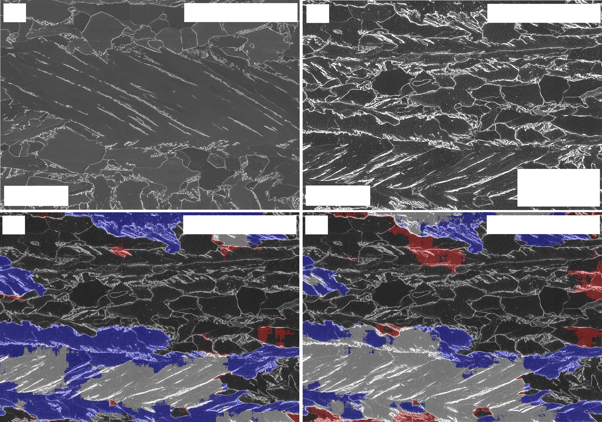
• Dual-phase steel constituents on SEM micrographs (martensite, bainite, pearlite, …).
• Fully Convolutional Net + superpixel max-voting.
• Prior SOTA: 48.9% → FCNN: 93.94%.
• Same images. No new physics — representation change alone.

Note

The 45-point jump is the headline of this whole unit.

Pause 30 seconds on the numbers. 48.9% → 93.94% on the same SEM images, by the same humans labelling. Read the numbers aloud. Don’t fill the silence.

What did not change. Same dataset, same physical evidence, same expert labels. The only knob turned was the encoding/representation. That is the entire argument of §1.

Anti-hype guardrail. Don’t generalise to “CNNs always win 45 points.” This is a single-dataset record. The lesson is the pattern (representation > metric), not the specific number.

Read the architecture left-to-right. Cropped constituent at native resolution → warped to 224×224 → VGG-style conv stack → fully connected → softmax over phase classes. Standard pre-2018 architecture, applied carefully — not an exotic novelty.

Take-home for the lecture. If they remember one slide today, this is the one.

09. Where Hand-Crafted Hits a Wall — A Wider View

CNN-based image retrieval on UHCS micrographs. A query micrograph (top-left) and the three nearest neighbours by CNN feature distance — same-class structures retrieved without any human-defined descriptor Holm, Elizabeth A. et al., (2020), doi:10.1007/s11661-020-06008-4.

Holm et al., MMTA 2020 — review Holm, Elizabeth A. et al., (2020), doi:10.1007/s11661-020-06008-4

• Surveys CV/ML across classification, semantic segmentation, object detection, instance segmentation.
• Pattern: where labels exist, learned representations match or beat hand-crafted features.
• The bottleneck has moved: from “which descriptor?” to “which labels and which split?”

Walk the image left-to-right. Top-left is the query, the other three are nearest neighbours by CNN feature distance. No human-defined descriptor. Same heat-treatment class without ever being told about heat treatments.

The deeper point. This is unsupervised structure discovery. The CNN was trained for classification on natural images and the embedding still clusters microstructures sensibly. Powerful.

Where the bottleneck moved. From “which descriptor?” to “which labels and which split?” — that shift is the unifying theme of §3+§4 and the failure mode catalogue of §5.

Reading list. Holm et al. 2020 is twenty pages, ~200 references, no math. Single best one-paper entry to this field for any motivated student.

10. The Paradigm Shift

	Classical	Modern (learned)
Input	Image \(\to\) metrics	Image / signal \(\to\) representation
Features	Hand-crafted, named	Learned (or correlation-based)
Bottleneck	Information loss	Data + compute + validation discipline

Ethics carry over

• Specimen splits, leakage, calibration — all unchanged.
• Scientist still owns labels, splits, metrics, physics checks Neuer, Michael et al., (2024).

§1 closing recap (30 seconds). Stereology compresses too hard. Learned representations preserve more. The professional duties — splits, leakage, calibration — do not change. End of motivation.

Anti-hype. “Let the network find features” does not remove responsibility for leakage, shift, or spurious correlations. §5 enumerates those obligations explicitly.

Pause for questions before §2. The technical content starts on the next slide; clear the room of motivation questions first.

§2 · Encoding Microstructure for ML

11. The Encoding Question

Before training: map microstructure to tensor \(\mathbf{X}\).

Principle: encoding upper-bounds what physics the hypothesis class can express Neuer, Michael et al., (2024).

Garbage encoding \(\Rightarrow\) garbage in, regardless of architecture.

Encoding	Shape	What the model sees
Hand-crafted	\(\mathbb{R}^D\), small	Pre-distilled features
\(S_2\) / patches	\(\mathbb{R}^{D'}\)	Correlations / local stats
Eigen-modes	\(\mathbb{R}^{K}\)	Linear modes of structure
Image + conv	\(\mathbb{R}^{H \times W \times C}\)	Spatial features (Unit 5)

Most underappreciated decision in materials ML. Choose wrong here and no architecture saves you. Worth saying aloud, slowly.

Why “upper-bound”. No model can learn physics that the encoding deletes. If you only feed mean grain size, no MLP — however deep — can learn weakest-link fracture. The encoding sets the ceiling; the architecture decides how close to the ceiling you get.

Show the table top-down. Each row keeps more morphological detail and each row demands more data. Going down the table = trading bias for variance. Same bias-variance language as Unit 3.

Forward signpost. The next six slides walk every row of this table — tabular, \(S_2\), eigen-modes, image, 1-D spectra, decision rule.

12. Tabular: Composition + Process

• Often no image in \(\mathbf{X}\):
  • Composition fractions in \(\mathbb{R}^{d_{\text{el}}}\).
  • Process: temperature, time, cooling rate, atmosphere.
  • History: ordered steps (embedded or binned).

MLP turf

• \(D \sim 10\)–\(50\), well-defined units.
• Standardise per train fold; freeze \((\mu, \sigma)\) at inference Neuer, Michael et al., (2024).
• Watch: mass fractions sum to 1 → drop one column or use compositional geometry.

The boring-but-strong baseline. A 20-D vector of composition + process beats most flashy CNN attempts when \(N \lesssim 500\) specimens. Tell students this before they over-engineer.

Concrete example. Steel UTS from C–Mn–Cr–Ni–Mo + tempering recipe — Calphad-grade benchmark, well-understood baseline. We use this for grading the easy half of Exercise 1.

Common student error. Composition fractions sum to 1 → covariance matrix is singular. They will hit this; flag it once now to save email later.

Connect. All of Unit 3 (cleaning, scaling, grouped CV) applies row-by-row to tabular materials data, unchanged.

13. Two-Point Statistics \(S_2\)

\[S_2(\mathbf{r}) = P\!\bigl(\text{phase}(\mathbf{x})=\alpha \,\wedge\, \text{phase}(\mathbf{x}+\mathbf{r})=\alpha\bigr)\]

• Translation-averaged correlation.
• Captures length scales, anisotropy, clustering — far more than one scalar, far less than full pixels Sandfeld, Stefan et al., (2024).

Why MLP-friendly

• Fixed-length vector after binning \(\mathbf{r}\) on a grid in the unit cell / ROI.
• Pairs naturally with standardised inputs (Unit 3).
• \(D \sim 10^2\)–\(10^3\) — tractable on materials sample counts.

Anchor in something they know. \(S_2\) is spatial covariance for phases. If they have seen the variogram from geostatistics, this is the same animal — just discrete labels instead of Gaussian fields.

Sanity check. $S_2() = $ phase fraction. So at the origin, \(S_2\) collapses to the ASTM phase-fraction number we left behind on slide 4. \(S_2\) is a strict generalisation of stereology — write that on the board.

Practical pitfall. Binning of \(\mathbf{r}\) and the ROI size both change \(S_2\) values quantitatively. Document them; treat them like any other preprocessing hyperparameter.

Pacing cue. Don’t rush this slide — the formula is dense. Two minutes minimum.

14. MKS Pipeline (Materials Knowledge Systems)

Typical chain

1. Segment / phase-label microstructure.
2. Compute \(S_2\) on a fixed grid of \(\mathbf{r}\).
3. Standardise correlation components using train statistics only (Unit 3).
4. Train MLP (or linear map) \(g_\theta(S_2) \approx\) property Sandfeld, Stefan et al., (2024).

Why it works

• Bakes in translation invariance before the net sees data.
• Keeps \(D\) in the hundreds — matches typical materials sample counts.
• Strong baseline before escalating to CNNs on raw pixels.

Historical context. This is the Kalidindi recipe — a body of work from Georgia Tech, ~20 years old. Robust, well-understood, the right starting point for a structure-property regression project.

Why the pipeline order matters. Standardise inside CV folds, never on the full dataset before splitting. Same Unit-3 hygiene as for tabular data — the names of the columns are different, the discipline is identical.

Forward signpost. Slide 26 shows a CNN beating MKS on composite stiffness. Slide 40 shows a CNN ⊕ \(S_2\) hybrid beating both. The story is “MKS is the baseline, not the ceiling.”

15. Eigen-Microstructures

Idea. Stack registered microstructure fields (phase indicator, orientation channels) into a design matrix; PCA on standardised columns yields dominant modes of structural variation — “eigen-microstructures.”

Why standardise first?

• Without it, PC1 often tracks brightness, thickness, detector gain — not microstructure.
• With per-feature z-scores fit on train only, PCs more often reflect shape variation Sandfeld, Stefan et al., (2024).

Connect: Unit 5 CNNs learn spatial features end-to-end; eigen-modes are the linear baseline to beat.

Analogy that lands. Same idea as eigenfaces from 1990s computer vision — but on phase-indicator fields instead of RGB faces. PC1 is the dominant direction of structural variation, not a face.

The standardisation trap. Without per-pixel z-scores, PC1 will track brightness, thickness, detector gain, vignetting — not microstructure. Show this on the board: a single misaligned bright background creates a fake “mode” that dominates everything.

Why it still matters in 2026. Eigen-microstructures are the linear baseline that students need to beat before claiming a CNN works. If \(N=80\) samples and the linear model already explains the test variance, the CNN adds nothing.

Pitfall. Alignment / cropping must be consistent across specimens — misregistration manufactures fake modes that look like signal.

16. Image as Tensor

• 2-D micrograph: \(\mathbf{X} \in \mathbb{R}^{H \times W \times C}\).
• 3-D tomography: \(\mathbf{X} \in \mathbb{R}^{D \times H \times W \times C}\).
• \(C\) = channels: BSE/SE, EBSD orientation Euler angles, EDS element maps.

MLP on flattened pixels?

• \(1024 \times 1024\) flattened → first dense layer ≈ \(10^9\) weights.
• With \(N \sim 100\) specimens: spurious correlations win.
• Solution: convolutional inductive bias (Unit 5).

Make the parameter blow-up visceral. \(1024 \times 1024 \times 3\) RGB ≈ \(3 \times 10^6\) inputs → first dense layer with 1000 hidden units = \(3 \times 10^9\) weights. With \(N=100\) specimens, that’s \(3 \times 10^7\) parameters per training example. No statistical signal survives that ratio.

Where channels come from in practice. BSE/SE for SEM, Euler-angle channels for EBSD, element maps for EDS, \(z\)-stacked tomography slices. Multi-channel from day one — students often forget the channel dimension.

Pre-empt the bad fix. Aggressive downsampling to make MLP tractable destroys fine porosity / dislocation contrast — that is physics loss, not a numerical trick.

Bridge. “On slide 45 we make this argument formal — and it is the cleanest single motivation for next week’s CNN lecture.”

17. Spectra as 1-D Signals

• XRD pattern, EELS edge, Raman spectrum: \(\mathbf{x} \in \mathbb{R}^{N_{\text{channels}}}\).
• Locality matters along the channel index — neighbouring bins describe the same peak.
• The convolutional inductive bias applies in 1-D too.

1-D CNN is the natural architecture

• Same shared weights, same locality argument as 2-D images.
• Preview: Park 2017 (slide 28) — phase ID with a 1-D CNN.

Note

“CNN” is not a synonym for “image network.”

Break the misconception now. If they finish today thinking “CNN = image network”, I have failed. Convolution is locality with shared weights. Anywhere data has local structure, convolution applies.

Cross-domain examples. Audio (1-D), ECG (1-D), time series (1-D), pixels (2-D), tomography volumes (3-D). Same inductive bias, different dimensionality.

Forward signpost. Slide 28 (Lee/Park 2020) is the payoff — a 1-D CNN identifies XRD phases at ~100% accuracy. That is the example to remember when “CNN” is mentioned next.

Connect. EELS, EDS, Raman analysis in Unit 10 reuse this same encoding. Today’s investment carries.

18. Encoding Decision Rule

Input type	Typical \(D\)	First-line model
Composition + process	10–50	MLP
Morphology scalars	5–50	MLP
\(S_2\) / MKS	\(10^2\)–\(10^3\)	MLP / shallow 1-D conv
1-D spectrum	\(10^3\)–\(10^4\)	1-D CNN
2-D micrograph	\(10^4\)–\(10^7\)	CNN (Unit 5)
3-D volume	\(10^6\)–\(10^9\)	3-D CNN / U-Net

Decision rule

• Start with the smallest \(\mathbf{X}\) that passes physics + grouped CV.
• Add representation capacity when grouped CV shows a persistent gap, not when train loss wants it McClarren, Ryan G., (2021).

Cheat-sheet slide. Tell them to take a phone photo. When they read a microstructure-ML paper next week, the first question is which row is this? — that single question filters most overhyped abstracts.

Decision rule, said plainly. Start at the top. Escalate one row only when grouped CV shows a persistent gap. Never escalate because train loss looks bad — that is over-fitting bait.

War story. Past student project: 200 JPEGs, jumped straight to ResNet, beautiful training curves, \(R^2 = 0.92\) on a random split. Specimen-level split: \(R^2 = 0.31\). The fix was not a bigger network; it was a smaller encoding and an honest split.

Section close. “End of theory. Now we look at what happens when you do this right.” → §3.

§3 · Application Gallery — Characterization

19. Gallery Overview — Characterization

Six task families

1. Classification (slide 20–21).
2. Segmentation (22–23).
3. Defect / feature detection (24–25).
4. Property regression from images (26–27).
5. Spectroscopy (28).
6. 3-D tomography (29).

Common pattern

raw signal  →  CNN  →  label / property

No hand-crafted descriptors. Same architecture family across SEM, EBSD, TEM, XRD, X-ray CT.

Frame the gallery. “I will show ten case studies in ~18 minutes — about 2 min each. Don’t try to memorise the numbers. Look for the pattern — slide 30 will pull it together.”

Active prompt to set up. “By slide 30, I want you to be able to fill in this template for any new paper: signal → encoding → architecture → loss → label.” Tell them now so they listen for it.

Pacing rule. If a case is generating questions, hold them to slide 30. We can’t lose budget here, §5 needs the time.

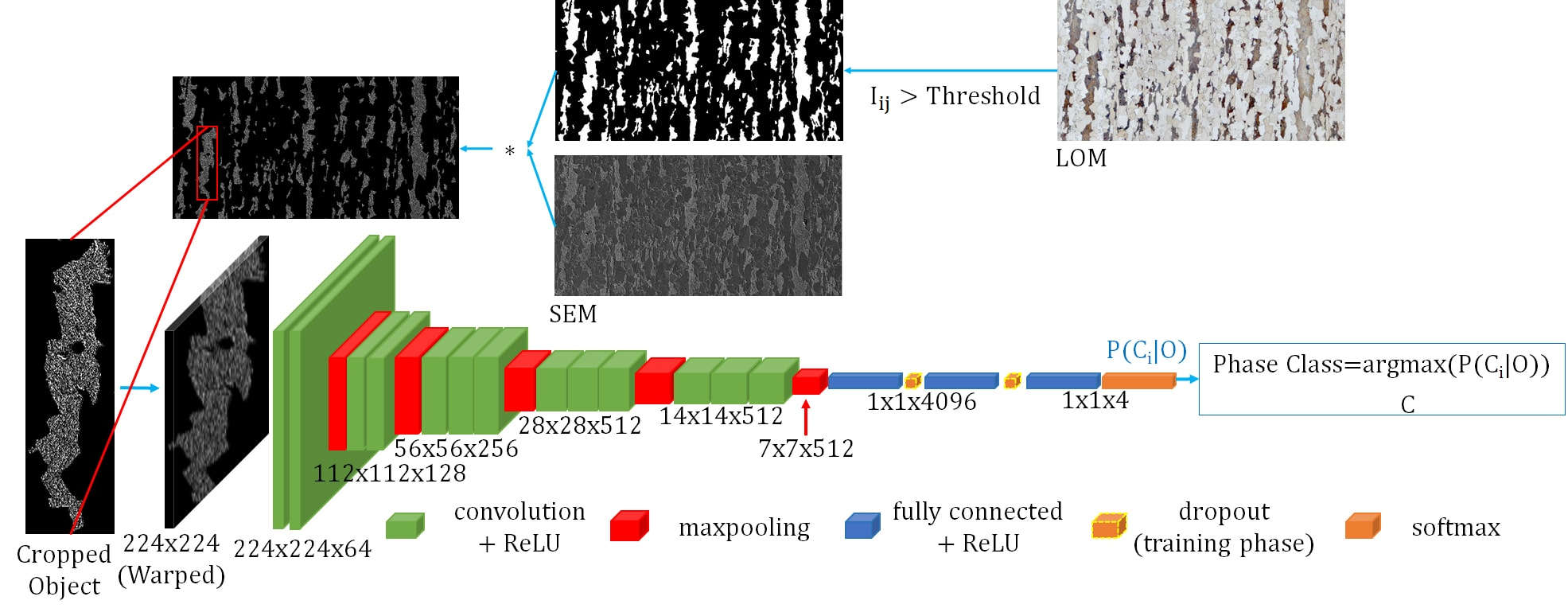
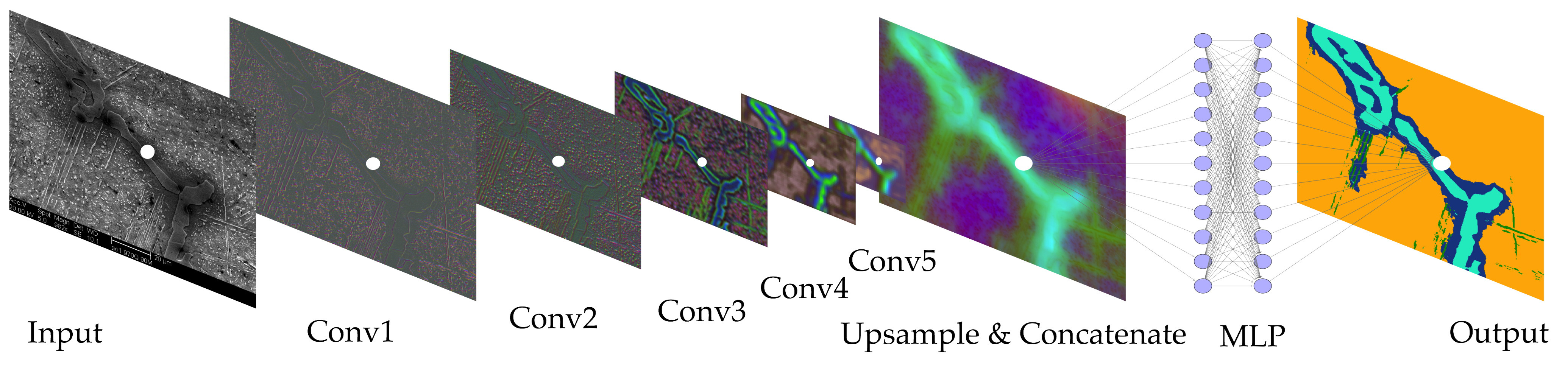
20. Case 1 — Steel Phase Classification (Azimi 2018)

Pixel-wise FCNN segmentation: SEM input → ground truth → predicted phase map (martensite, bainite, pearlite, ferrite). Same network, four different microstructures Azimi, Seyed Majid et al., (2018), doi:10.1038/s41598-018-20037-5.

• Task. Classify constituents in dual-phase steel SEM micrographs.
• Method. Fully Convolutional Net + max-voting on superpixels.
• Data. Thousands of SEM tiles, expert-labelled.
• Result. 93.94% vs prior SOTA 48.9%.
• Lesson. Representation change alone unlocks the 45-pt jump.

Reframe. Slide 8 showed the headline number; this slide shows the output. The image is pixel-perfect phase maps, not just an image-level label.

Hands-on anchor. “Compare to your last metallography lab. How long did it take you to label one micrograph? Hours. This network does thousands per minute, at the same expert quality.”

Read the figure. Four columns = four different microstructures. Three rows = SEM input / ground truth / FCNN prediction. Walk one column top-to-bottom — students see the pipeline at a glance.

Stake. Pixel-level segmentation is what enables automated metallography in industry — the entire downstream stereology workflow runs on these maps. This is the production payoff of slide 8.

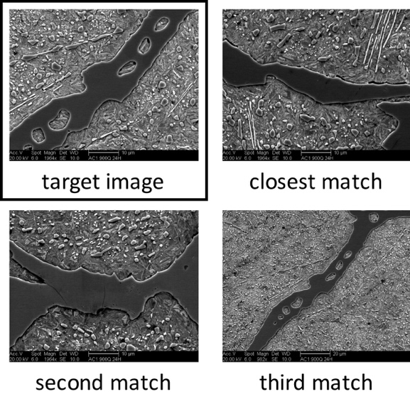
21. Case 2 — UHCS Microstructure Manifold (DeCost & Holm)

2017 — Microstructure manifold. UHCS micrographs embedded by CNN features cluster spontaneously by heat-treatment class — no labels used to position them DeCost, Brian L. et al., (2017), doi:10.1016/j.actamat.2017.05.014.

2019 — High-throughput segmentation. Input SEM → CNN encoder (Conv1–5) + upsampling → per-pixel constituent map DeCost, Brian L. et al., (2019), doi:10.1017/S1431927618015635.

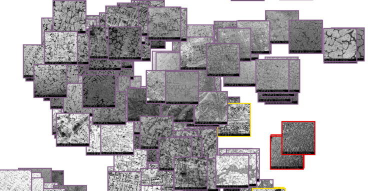
• Dataset. 961 public UHCS micrographs (materialsdata.nist.gov).
• Lesson. Pretrained CNN features cluster phase classes without labels — a transfer-learning preview (Unit 6) and the basis for Exercise 1.

The “MNIST of microstructures.” 961 SEM micrographs, public, NIST-curated. Doable on a laptop. If anyone is starting a project, start here.

Two-paper story to tell. 2017: CNN features cluster better than the human-engineered SIFT features they replaced. 2019: segmentation is now a one-line script. Two years apart, same dataset, two papers — that’s the pace of this field.

Read the left figure carefully. The 2-D map is unsupervised. No heat-treatment label was used to position the micrographs — the network learned the structure from images alone, and class identity emerged.

Exercise hook. Exercise 1 reproduces a small slice of this. Tell them the dataset URL aloud — materialsdata.nist.gov.

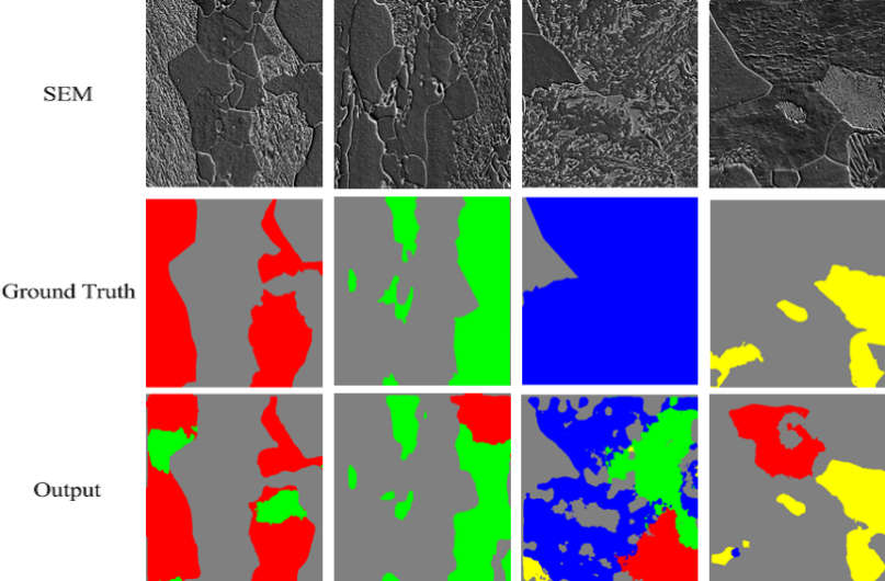
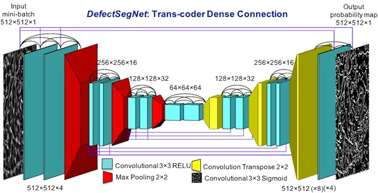
22. Case 3 — U-Net for EBSD Phase Segmentation

Inputs. Band-slope (BS), grain-boundary overlay, KAM map, manual labels — the EBSD-derived channels feeding the U-Net Martinez Ostormujof, T. et al., (2022), doi:10.1016/j.matchar.2021.111638.

Cross-temperature results. Three test temperatures (T1–T3); top: BS micrograph; middle: prediction with accuracy 99.3% / 98.5% / 97.2%; bottom: error map Martinez Ostormujof, T. et al., (2022), doi:10.1016/j.matchar.2021.111638.

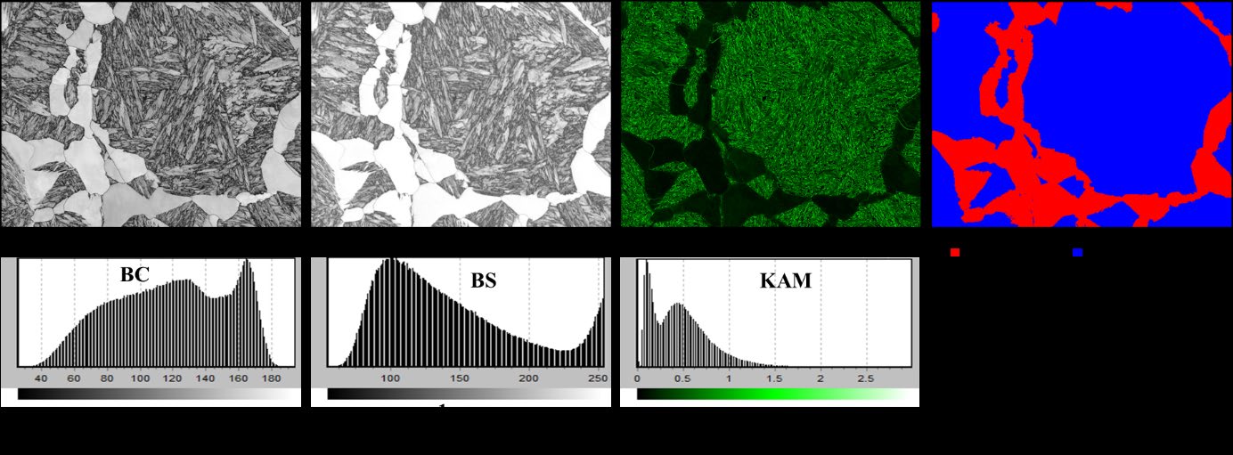
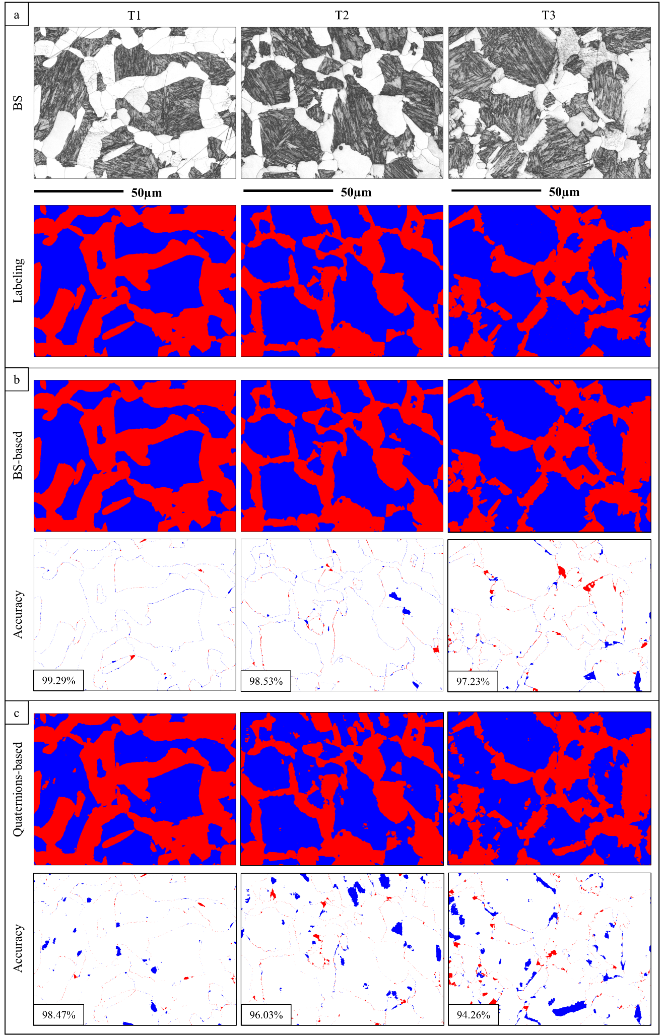
• Task. Pixel-level martensite / ferrite-bainite segmentation across three tempering conditions.
• Lesson. A standard U-Net on a single grayscale BS channel can reach the EBSD-quaternion baseline if augmentation is honest.

Why this case matters in industry. EBSD is minutes per frame; band-slope (BS) imaging is seconds. Train the U-Net with EBSD-grade labels, deploy it on BS-only data at inference: ~100× throughput at the same quality.

Read the figure. Left = the four input/label channels. Right = three test temperatures (T1, T2, T3) with prediction accuracy 99.3% / 98.5% / 97.2% — meaningful generalisation across processing conditions, not just within one condition.

Pitfall to flag. Achievable accuracy is bounded by annotator agreement — measure inter-annotator variance before chasing the last 1%. Past that floor, more capacity buys nothing (we will see this again on slide 25).

Take-home. “EBSD-grade labels at training time → BS-imaging throughput at deployment time” — write that pattern down.

23. Case 4 — Complex Microstructure Inference (Durmaz et al. 2021)

Multi-modal training data. Light-optical micrograph (LOM, top) and SEM (middle) of the same area, co-registered with EBSD-derived bainite-instance overlays (bottom) Durmaz, Ali Riza et al., (2021), doi:10.1038/s41467-021-26565-5.

Lath-bainite instance segmentation. Top row: LOM input + SEM input; bottom row: per-instance prediction colored by lath family Durmaz, Ali Riza et al., (2021), doi:10.1038/s41467-021-26565-5.

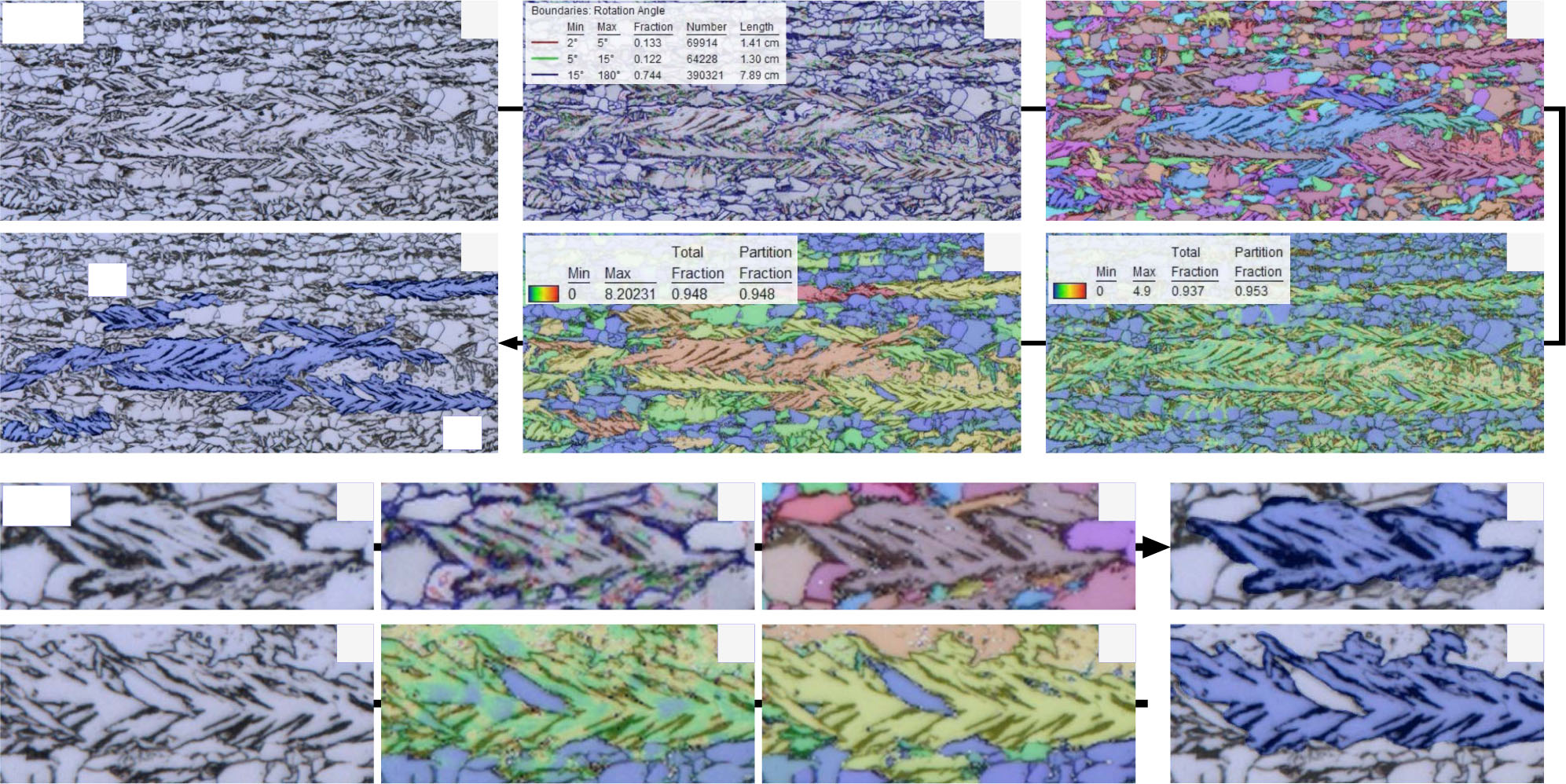
• Method. U-Net (semantic) + Mask R-CNN (instance) trained on EBSD-derived ground truth, deployed on LOM/SEM only at inference.
• Lesson. EBSD-grade labels at training time → optical-microscopy throughput at inference time.

The historical pain. Distinguishing ferrite / pearlite / bainite / martensite jointly is the canonical hard problem in metallography — needed by Fraunhofer and by every steel mill quality lab. This paper resolves it for the first time at production accuracy.

Why multi-modal helps. LOM, SEM, and EBSD see different physics — etched relief vs electron contrast vs orientation. Co-registered, they constrain the segmentation more than any one modality can alone.

Read the figure right. Training: uses EBSD-derived ground truth (which is slow but accurate). Inference: runs on LOM/SEM only. That asymmetry is the practical innovation — fast deployment, expensive labels.

Connect. Cross-instrument robustness here previews the lab-shift discussion on slide 42.

24. Case 5 — TEM Dislocation Segmentation (Govind et al. 2024)

Simulated TEM dislocation training image — physics-based contrast with controllable label density Govind, Kishan et al., (2024), doi:10.1088/2632-2153/ad1a4e.

Real experimental TEM micrograph — dislocation arcs against grain background Govind, Kishan et al., (2024), doi:10.1088/2632-2153/ad1a4e.

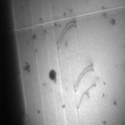
• Task. Instance segmentation of dislocations in TEM.
• Method. YOLO-style + U-Net trained on simulated dislocation images, evaluated on real experiments.
• Lesson. Simulation-augmented training bypasses the “never enough labels” bottleneck — standard wherever physics simulators are mature.

The pain quantified. Hand-labelling dislocations in TEM costs roughly one postdoc-week per micrograph. With \(N=10^4\) training examples needed, that is centuries of postdoc time. Untenable.

The trick. Train on simulated TEM images — physics-based contrast, Tomic-Mølnar dislocation models, controllable label density. Real images at test time only. The simulator becomes the labelling machine.

Read the figure side-by-side. Simulated (left) and real (right) look strikingly similar at TEM resolution — that visual proximity is what makes the transfer work.

Pattern to flag. Same simulation-augmented training appears on slide 29 (Müller battery). Tell students: “This is the answer to small-\(N\) in 2026.” Wherever a physics simulator exists, the labelling problem inverts from cost-bound to compute-bound.

Project hook. Dislocation databases and TEM simulators are public. Low barrier for student projects.

25. Case 6 — STEM Defects in Irradiated Steels (Roberts 2019)

DefectSegNet — encoder–decoder U-Net with trans-coder dense skip connections; 512×512 input → per-pixel probability map Roberts, Graham et al., (2019), doi:10.1038/s41598-019-49105-0.

Per-class results: input STEM (DCI), ground truth, prediction, and overlay-comparison for precipitates and voids Roberts, Graham et al., (2019), doi:10.1038/s41598-019-49105-0.

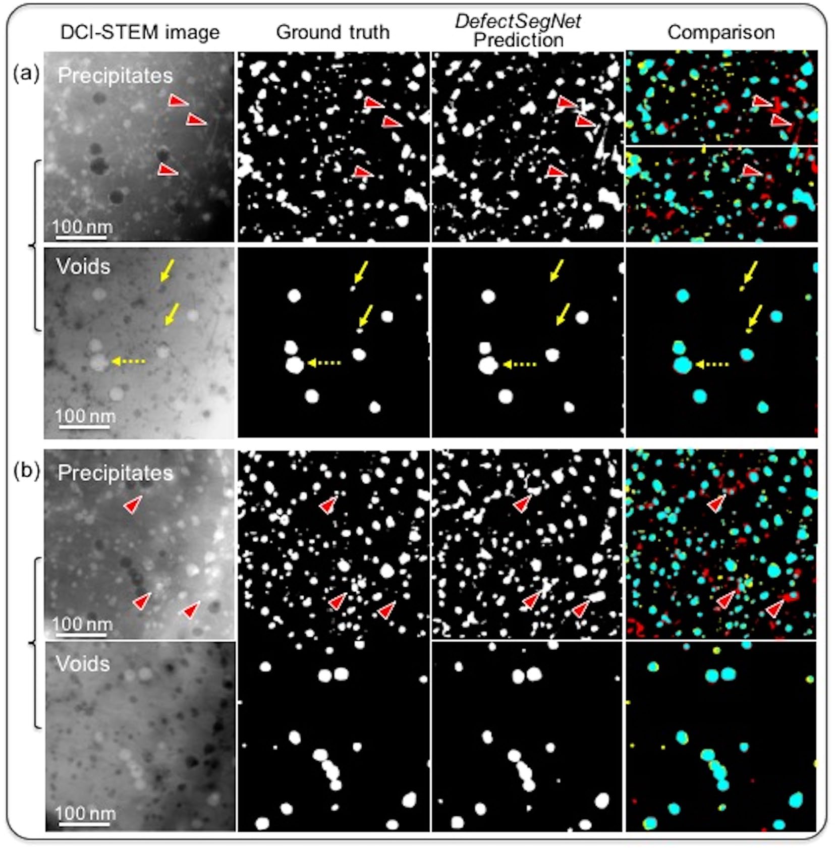
• Task. Semantic segmentation of voids, dislocation loops, precipitates in irradiated steels.
• Result. ~85% IoU — matches inter-annotator variability.
• Lesson. Once you hit the annotator floor, more model capacity buys nothing.

Real-world urgency. This is reactor steel post-irradiation. Worldwide, a handful of people can label voids and dislocation loops in STEM at expert level. The CNN reaches their accuracy on hundreds of training images.

Read the architecture. Left figure = U-Net with dense skip connections. Standard pattern: encoder downsamples, decoder upsamples, skip connections preserve fine-scale features. This is the off-the-shelf architecture for almost every materials segmentation task.

Right figure read. Four columns = STEM input / human label / CNN prediction / overlay-difference. The “comparison” column highlights the few pixels where the network disagrees — and most of those are at object boundaries where humans also disagree.

Hard rule for projects. Once you hit annotator-floor performance, more model capacity buys nothing. Invest in better labels or new tasks. This is one of the most expensive lessons in this field.

26. Case 7 — 3-D-CNN Composite Stiffness from RVEs

• Task. Predict effective stiffness tensor of two-phase composites from voxelated RVEs Yang, Zijiang et al., (2018), doi:10.1016/j.commatsci.2018.05.014.
• Method. 3-D CNN trained on FE-homogenised stiffness labels.

• Result. >40% accuracy improvement over hand-engineered descriptors at a fraction of the FE cost.
• Lesson. CNNs can act as homogenisation surrogates inside design loops where each FE call is too expensive.

Switch of register. Slides 20–25 were about classification / segmentation — labels from images. From here on it’s regression — physical quantities from images.

The economic stake. A single FE homogenisation call takes minutes; CNN forward pass takes milliseconds. In a design loop that searches over \(10^6\) candidate microstructures, the FE inner solve is the bottleneck. CNN-as-surrogate is what makes inverse design tractable.

Important nuance. The CNN is not replacing FE forever — it replaces FE inside the inner loop, with FE used to generate training data and to verify candidate winners. Nobody trusts a black-box surrogate alone in 2026.

Connect. Same “CNN as physics surrogate” pattern reappears on slide 36 (Mianroodi crystal plasticity). Difference: Yang predicts a scalar (stiffness); Mianroodi predicts a field (per-voxel stress).

27. Case 8 — Yield-Surface Prediction from Microstructure

• Task. Predict the full yield surface (not a single scalar) from a microstructure image Heidenreich, Julian N. et al., (2023), doi:10.1016/j.ijplas.2022.103506.
• Method. CNN regression with a multi-output head producing yield-surface coefficients.

• Lesson. A learned representation lets one model output functional properties — anisotropic yield, stress-strain curves, dispersion relations.
• Significance. Moves CNNs from “label predictors” to “constitutive surrogates.”

Why this case is different. Most CNN papers predict a scalar (a label, a stiffness, a temperature). This one predicts a surface in stress space — a much higher-information output. Same backbone, different head.

The architectural lesson. Output structure is a deliberate design choice. Vector head → labels; matrix head → covariance / stiffness tensor; function head → yield surface, stress-strain curve, dispersion relation. Each is just a different last layer.

Engineering consequence. This is what unlocks ML-driven constitutive modelling — replacing hand-crafted yield functions (von Mises, Hill, Yld2000) with a learned surrogate per microstructure. A genuinely new capability, not just a faster computation.

28. Case 9 — Lee/Park et al. 2020 — XRD Phase ID with 1-D CNN

1-D CNN architecture. XRD pattern (top-left) → stack of 1-D conv layers → flatten → fully-connected → multi-head outputs (existence + fraction of each phase) Lee, Jin-Woong et al., (2020), doi:10.1038/s41467-019-13749-3.

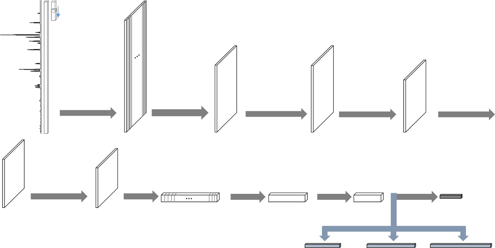
• Task. Phase ID in multi-phase inorganic mixtures from XRD.
• Train on simulation, test on real. ~\(10^5\) patterns from ICSD with augmentation for strain, texture, peak broadening.
• Result. ~100% phase ID; ~86% three-phase quantification on real experiments.
• Lesson. CNN \(\neq\) image network — convolution applies wherever there is locality (peak shape along \(2\theta\)).

This is the slide I want them to remember when they hear “CNN” next. Read the architecture aloud: XRD pattern → 1-D conv layers → fully-connected → multi-head outputs (one per phase). No image anywhere. This is the strongest “CNN ≠ image network” example I have.

Why train on simulation, test on real. The Inorganic Crystal Structure Database has \(\sim 10^5\) known phases — that is the catalogue. Each entry simulates exactly. Real experimental XRD with manual phase ID is at most \(\sim 10^4\) samples worldwide. Training on simulation is the only practical strategy.

The augmentation that makes it work. Strain (peak shifts), texture (peak intensities), particle size (peak broadening) — three physics-driven augmentations. Without them, the model overfits to noise-free idealised patterns and breaks on real data.

Pedagogy hook. Translation-equivariance + weight sharing is the inductive bias. It applies along \(2\theta\) here, along time in audio, along space in pixels, along voxels in tomography. Same idea, different axis.

29. Case 10 — 3-D U-Net for Li-ion Electrode Tomography

X-ray nano-CT input → 3-class 3-D segmentation. Input volume (top), reconstruction (right), final segmentation: active material (grey), carbon-binder (orange), pore (blue) Müller, Simon et al., (2021), doi:10.1038/s41467-021-26480-9.

Per-slice quality. Same input, four output variants — only the deep-learning column recovers the carbon-binder phase consistently Müller, Simon et al., (2021), doi:10.1038/s41467-021-26480-9.

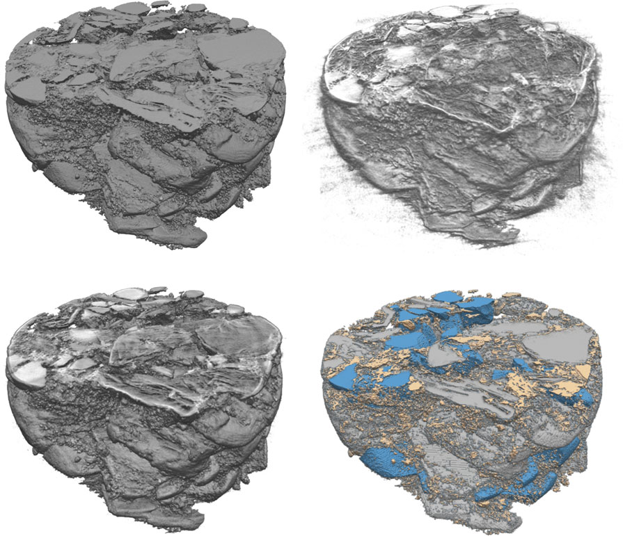
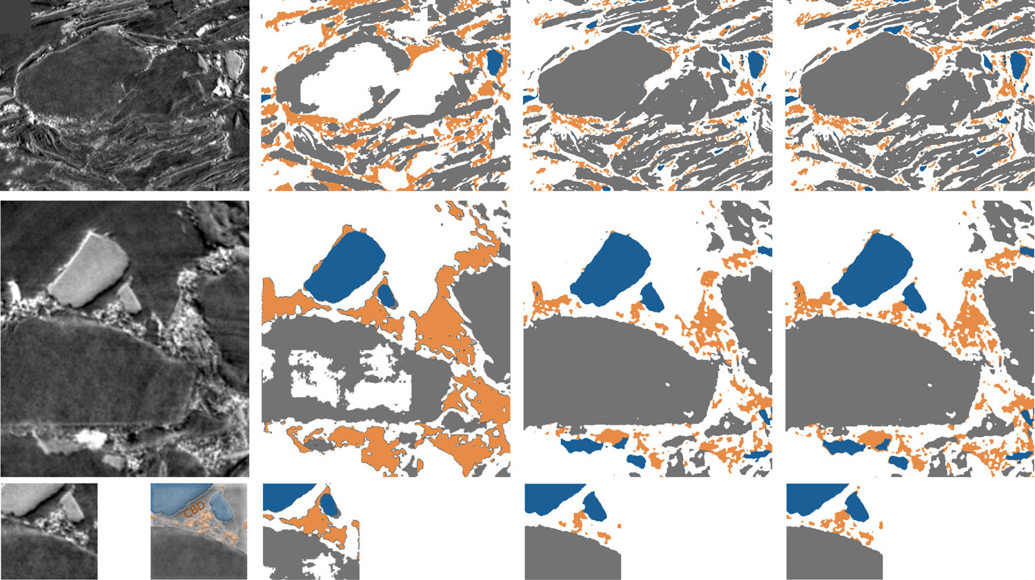
• Method. 3-D U-Net trained partly on synthetic electrodes with known voxel-level ground truth.
• Lesson. Carbon-binder vs pore has near-zero contrast — thresholding fails; simulation-augmented CNN succeeds.

The unsolvable-by-thresholding case. Carbon-binder and pore have nearly identical X-ray attenuation. Histogram-thresholding cannot separate them — the contrast is below detector noise. This is the case where classical CV is impossible in principle, not just imprecise.

How the CNN escapes. Trained on synthetic electrodes generated by physical packing simulators, where every voxel’s true label is known. The network learns the spatial signature of carbon-binder — its texture and connectivity — that survives even when intensity does not.

Read the right figure. Same input slice, four different segmentation methods. Only the deep-learning column recovers the carbon-binder phase consistently. Make this point aloud — students often skip the comparison columns.

Pattern reinforcement. Same simulation-augmented training as slide 24 (dislocations). Two papers, two domains, identical recipe. That is what we mean by “common toolkit”.

30. Characterization Gallery Recap

Same recipe across ten cases

• raw signal \(\to\) CNN \(\to\) label / property.
• Tasks: classification, segmentation, regression, retrieval.
• Domains: SEM, EBSD, TEM, STEM, XRD, X-ray CT.

What changed across cases

• The encoding (\(\mathbf{X}\)).
• The labels (\(y\)).
• The head of the network.

What did not change

• The convolutional inductive bias.
• The discipline (specimen splits, calibration, shift testing).

Active recall. Don’t read the slide. Ask: “What was common to all ten cases?” Wait. Take an answer. Then reveal the recipe.

Reinforce the abstraction. Encoding, labels, head — these change from paper to paper. Convolutional inductive bias and the Unit-3 discipline (splits, leakage, calibration) — these do not change. Knowing that distinction is what separates fluent paper-readers from beginners.

Transition. “§3 was characterization — what we measure after the part is made. §4 is processing — what we measure while it is being made. Same recipe, faster clock.”

§4 · Application Gallery — Processing

31. Gallery Overview — Processing

Six cases spanning:

• In-situ AM monitoring (32–33).
• Real-time welding inspection (34–35).
• CNNs as physics surrogates (36).
• End-to-end PSP closure (37).

Pattern

process sensor  →  CNN  →  quality
                            decision

The time scale changes: characterization is offline, processing is online — sometimes at video rate.

The fundamental shift. Characterization runs offline — pretty pictures, hours per analysis. Processing runs online — pretty pictures stream at video rate, decisions in milliseconds. The metrics that matter change accordingly.

New first-class metrics. Latency (ms-per-frame), throughput (frames-per-second), false-positive cost (one false alarm halts the build). Pure accuracy is necessary but no longer sufficient in §4.

Concrete pacing reframe. “I will compress §4 to ~12 minutes — six cases, ~2 min each. Faster than §3 because the recipe is the same; only the deployment context shifts.”

32. Case 11 — LPBF Powder-Bed Quality (Xception Transfer Learning)

• Task. Classify powder-bed defects (balling, incomplete spreading, groove, ridge, spatters, protruding part, scattered powder, homogeneous) from line-sensor recoater images during LPBF Fischer, Felix Gabriel et al., (2022), doi:10.1016/j.matdes.2022.111029.
• Method. Xception pretrained on ImageNet, fine-tuned on a Fraunhofer-ILT dataset acquired under coaxial / dark-field / diffuse lighting.

• Result. 99.15% classification accuracy across seven classes (dark-field condition); per-class F1 between 97.85% and 99.71%.
• Lesson. ImageNet pretraining transfers astonishingly well even to grayscale recoater frames — a clean transfer-learning teaser for Unit 6.

The “magic” worth questioning. Xception was pretrained on ImageNet — cats, dogs, cars, no powder beds. Yet its features transfer to grayscale recoater images at 99% accuracy. Why?

Why it works. Low-level CNN filters learn edges, gradients, textures, blob detectors — domain-agnostic primitives. High-level filters learn class-specific concepts (cat-ear, car-wheel). Materials tasks need the low-level features, which transfer freely.

Forward signpost. This is the cleanest transfer-learning teaser in the lecture. Unit 6 picks up the formal treatment — fine-tuning, frozen backbones, domain adaptation.

Critical pitfall to flag. Held-out frames from the same build \(\neq\) held-out builds. The 99.15% number is on within-build held-out frames. Probe build-level evaluation before claiming production readiness — this is the same specimen-split issue from Unit 3, just renamed.

33. Case 12 — Thermographic Porosity Prediction in LPBF

Sensing geometry. SWIR camera images the melt pool from above; sub-surface keyhole pores form below the visible track Oster, Simon et al., (2024), doi:10.1007/s10845-023-02117-0.

Specimen used for ground truth. LPBF Inconel 718 staircase sample — thermography during build, post-build µCT defines per-voxel porosity labels Oster, Simon et al., (2024), doi:10.1007/s10845-023-02117-0.

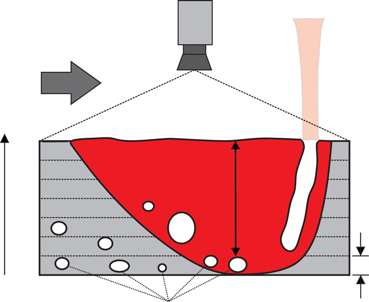
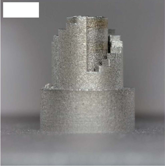
• Method. Multi-layer thermographic feature stack → supervised CNN classifier; CT ground truth.
• Result. Accuracy ~0.96, F1 ~0.86 for keyhole porosity in small sub-volumes.
• Lesson. Thermal history is a proxy for porosity — CNNs decode it densely, below the resolution of point pyrometers.

The proxy chain to call out. Thermal history → cooling rate → solidification physics → porosity. The CNN learns the entire chain implicitly — students should not infer it learned physics, only that thermal images carry enough information for the prediction.

Read the schematic. Camera (top) → melt pool (red) → keyhole pore (small white circles below the surface). Pores form below the visible track — that’s why the prediction problem is hard and why thermographic time-series are needed, not just one snapshot.

Why this is hard in the real world. Camera focus drifts, accelerating-voltage changes, exposure compensation kicks in mid-build. Many AM-monitoring projects fail not at the model but at the SOP. Read this aloud: “The hardest problem is keeping the camera the same camera.”

Connect. Same proxy logic powers Unit 7 (process time-series) — temperatures, currents, vibrations as proxies for state we cannot measure directly.

34. Case 13 — Real-Time FSW U-Net at ~25 fps

• Task. Surface defect segmentation + weld-width geometry in friction-stir welding Loganathan, Naveen et al., (2026), doi:10.1016/j.jmsy.2026.01.007.
• Method. U-Net optimised for on-device inference at video rate.

• Result. ~25 fps continuous inference; defect area + weld width streamed to closed-loop controller.
• Lesson. CNNs are now fast enough for in-line process control — not just offline metrology.

Why 25 fps is the headline, not the accuracy. Video rate enables closed-loop control — defect detected → laser power adjusted → next pass corrected. Anything slower is post-mortem inspection. The factor-of-10 speed-up is what changes the engineering use case.

The hardware reality. 25 fps + on-device inference = embedded GPU or NPU at the welder. Not a cloud round-trip. This is why latency, model size, and quantisation matter as much as accuracy in production CNNs.

Forward signpost. Unit 11 (automation) revisits this in depth — model compression, quantisation, deployment hardware. Today’s takeaway: in 2026, CNNs are fast enough for in-line process control. That was unthinkable in 2018.

35. Case 14 — Radiographic Weld Inspection (CNN-ViT)

End-to-end pipeline. Data → preprocessing → comparative training of (a) CNN baseline and (b) hybrid CNN-ViT (CNN backbone + patch tokenization + transformer encoder) → testing → explainability layer with Grad-CAM and self-attention maps Parmar, Kumar et al., (2026), doi:10.1038/s41598-026-44874-x.

Misclassification analysis with Grad-CAM. Original radiographs (top), expert ROIs (middle), and Grad-CAM heatmaps (bottom) for the four classes — the explainability layer reveals where the network looked when it got the answer wrong Parmar, Kumar et al., (2026), doi:10.1038/s41598-026-44874-x.

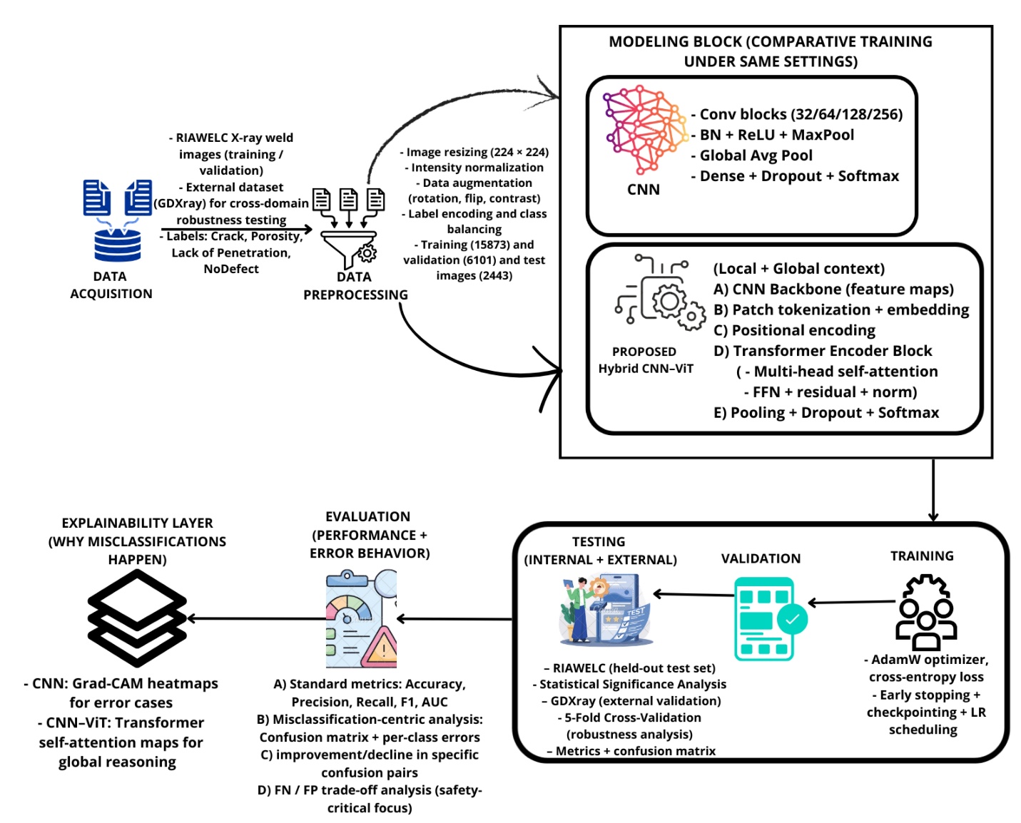
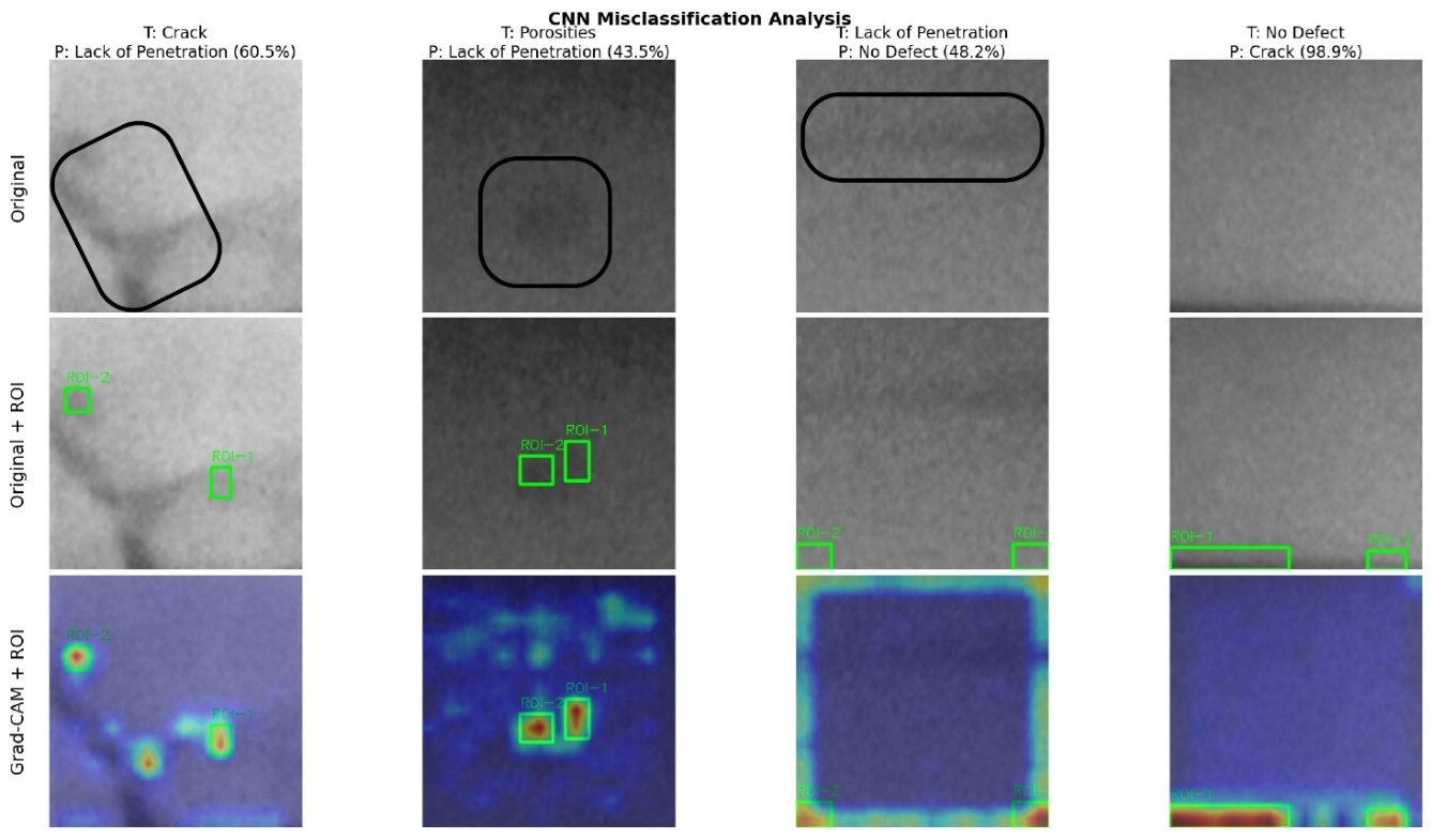
• Result. CNN-ViT 98.56% vs CNN baseline 97.90%; ~31% reduction in misclassification rate.
• Lesson. Hybrid CNN + ViT = local CNN features + global ViT context, with auditable Grad-CAM evidence per decision — a regulatory-grade design.

The non-negotiable backdrop. ASME IX, AWS D1.1 and similar welding codes require interpretability for inspection automation. A pure CNN that says “crack” with 99% confidence is not deployable without per-decision evidence. That regulatory floor — not curiosity — drives interpretability research in industry.

Architecture story. CNN backbone extracts local features (defect-level texture). Vision Transformer head re-aggregates patches with self-attention for global context (relating a crack to the surrounding weld geometry). Hybrid = local + global = best of both.

Read the right figure carefully. Top row: original radiographs. Middle: expert-marked ROIs. Bottom: Grad-CAM heatmap. The fourth column is fascinating — the network was wrong (predicted ‘Crack’ for an actually-defect-free image, with 98.9% confidence). The Grad-CAM map shows it latched onto the background frame, not the weld. This is exactly the kind of failure interpretability catches — and a pure-accuracy metric hides.

Take-home. Interpretability is a deployment requirement now, not a research nice-to-have.

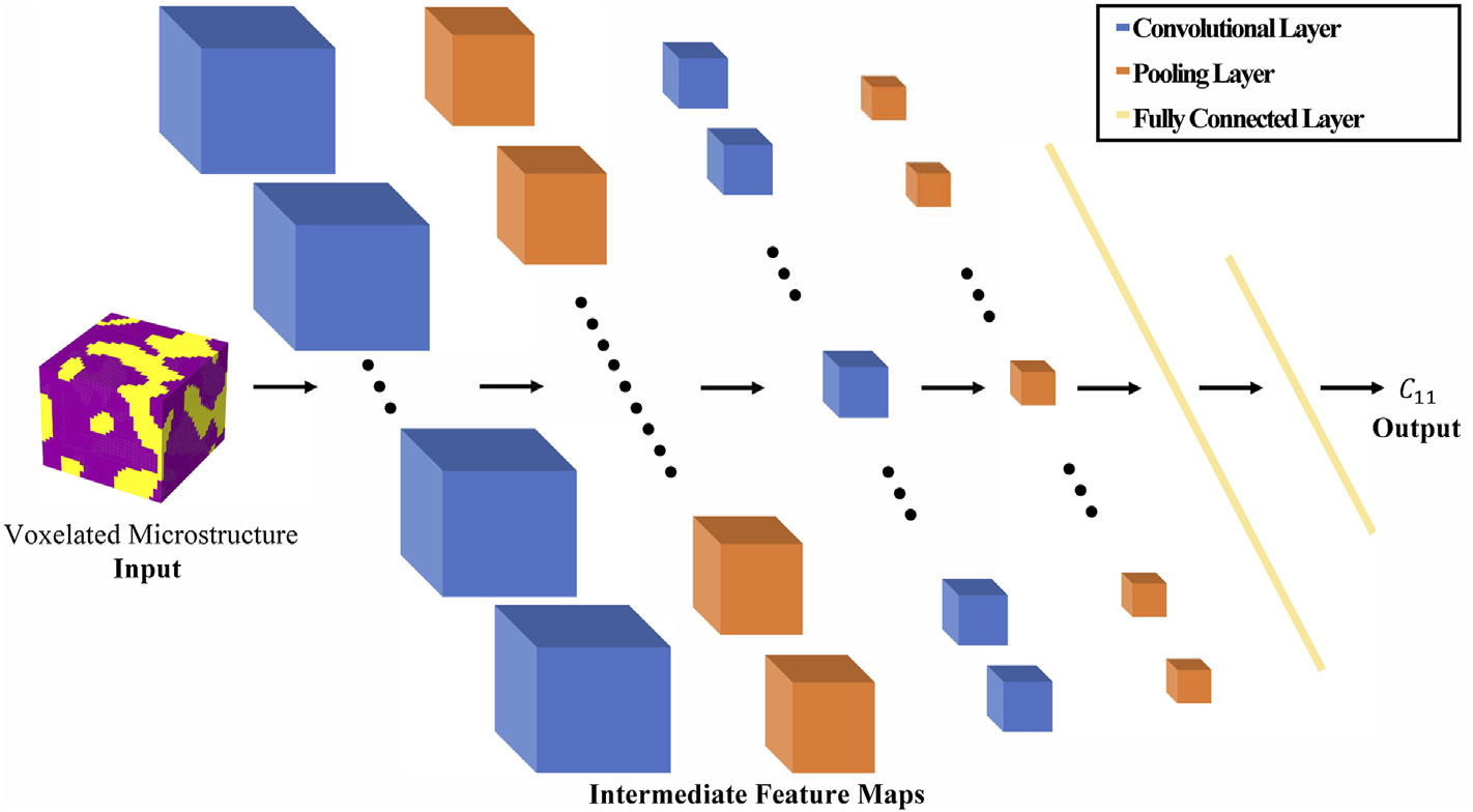
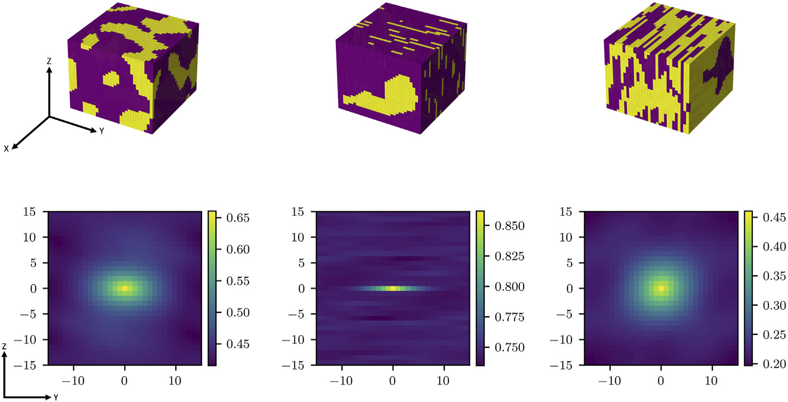
36. Case 15 — CNN as Crystal-Plasticity Surrogate

Voronoi grain RVEs — three test microstructures. Row (a) DAMASK FE ground truth \(S_\mathrm{vM}\), (b) CNN prediction, (c) error map; field-level agreement to within ±0.4 GPa Mianroodi, Jaber Rezaei et al., (2021), doi:10.1038/s41524-021-00571-z.

Inclusion shape generalisation — circle, square, diamond, divided square. Same CNN extrapolates to morphologies it never saw during training Mianroodi, Jaber Rezaei et al., (2021), doi:10.1038/s41524-021-00571-z.

• Method. 3-D CNN trained on CPFEM ground truth; orders of magnitude faster at inference.
• Lesson. CNN now a viable surrogate inside design loops — replaces FE inner solves wherever speed matters more than the last fraction of a percent.

The vital comparison with slide 26. Yang predicted a scalar \(C_{11}\) — one number per microstructure. Mianroodi predicts a field \(S_{vM}(\mathbf{x})\) — a value at every voxel. Same backbone, very different output capacity.

Why field-level prediction matters. Failure initiates locally — at one grain boundary, one pore, one stress concentration. Predicting only the average misses the failure-initiating site. Field-level surrogates can find these hot spots; scalar surrogates by construction cannot.

Read the figures. Left: three Voronoi RVEs, each with FE ground truth (a) / CNN prediction (b) / error map (c). Field-level agreement to ±0.4 GPa across the whole RVE. Right: same network on inclusion shapes (circle / square / diamond / divided square) it never saw in training — generalisation across morphology, not just within distribution.

Anti-hype. This is replacing FE inner solves where speed wins — not replacing FE forever. CNN training data still came from FE; CNN winners are still verified by FE. The surrogate is a budget tool, not a truth oracle.

37. Case 16 — End-to-End PSP Closure

Two CNNs in series

• Each CNN trained independently, then chained at inference.
• Lesson. The PSPP backbone of the course is now fully learnable end-to-end Sandfeld, Stefan et al., (2024).
• Caveat. Errors compound across the chain — Unit 12 will revisit uncertainty propagation.

The horizon, made explicit. This is the vision of materials informatics: process parameters → CNN-1 → predicted microstructure → CNN-2 → predicted property. Today’s case studies are the building blocks; this slide is the destination.

Walk the diagram. Left = process knobs (laser power, scan speed, atmosphere). Middle = predicted microstructure (the orange box — spatial output, not a label). Right = predicted property (strength, hardness, elongation).

The compounding-error caveat. CNN-1 has uncertainty \(\sigma_1\). CNN-2 has uncertainty \(\sigma_2\). Errors compound — naïvely chaining them gives optimistic confidence intervals. Unit 12 picks up uncertainty propagation seriously.

Active prompt. “Show of hands — how many groups in this room have CNN-1 in production? CNN-2? Both chained?” Tells you who is actually doing this.

38. Processing Gallery Recap

Six cases, same toolkit

• Cameras (LPBF, FSW), thermographs, radiographs, RVEs.
• Same convolutional inductive bias as in characterization.

Common ceiling

• Performance is bounded by labels and SOPs, not architectures.
• The model is rarely the limiting factor in 2026.

Active recall (mirror slide 30). Don’t read it. Ask: “What was common to all six cases this section?” Take an answer. Reveal.

The unifying point. In 2026, the CNN is rarely the bottleneck. Labels and SOPs are. If a project fails, look there before adding model capacity.

Tonal shift to set up §5. “We’ve now seen sixteen cases where it works. The next eight slides are the ways it looks like it works but doesn’t. Pay closer attention here than to anything else today.”

§5 · The Pattern + Pitfalls

39. The Common Pattern

All sixteen cases fit:

Raw signal   →  Encoding   →  CNN
   →  Loss   →  Label / property

• The architecture family is shared.
• The encoding and deployment unit decide the project.

What still varies

• \(\mathbf{X}\) — pixels, voxels, spectra, sensor streams.
• \(y\) — class, mask, scalar, function.
• Loss — cross-entropy, IoU, MSE, calibrated probabilistic.
• Split — by specimen / build / day / instrument.

The diagram is the takeaway of the whole lecture. If they remember one figure: signal → encoding → CNN → loss → label. Every paper in this whole field fits this template.

How to use it as a paper-reading aid. When they read a new paper next week, pause and identify each box. Most weak papers fail to specify the encoding choice or the splitting strategy. That hole is where the work is hiding.

Active prompt. “Pick a paper from your bibliography. In one sentence each: what’s \(\mathbf{X}\)? What’s \(y\)? What’s the loss? How is the data split?” If they can’t answer all four after a careful read, the paper is incomplete.

Connect. This is the ML equivalent of the “process → structure → property” PSPP backbone — a meta-frame that organises the whole field.

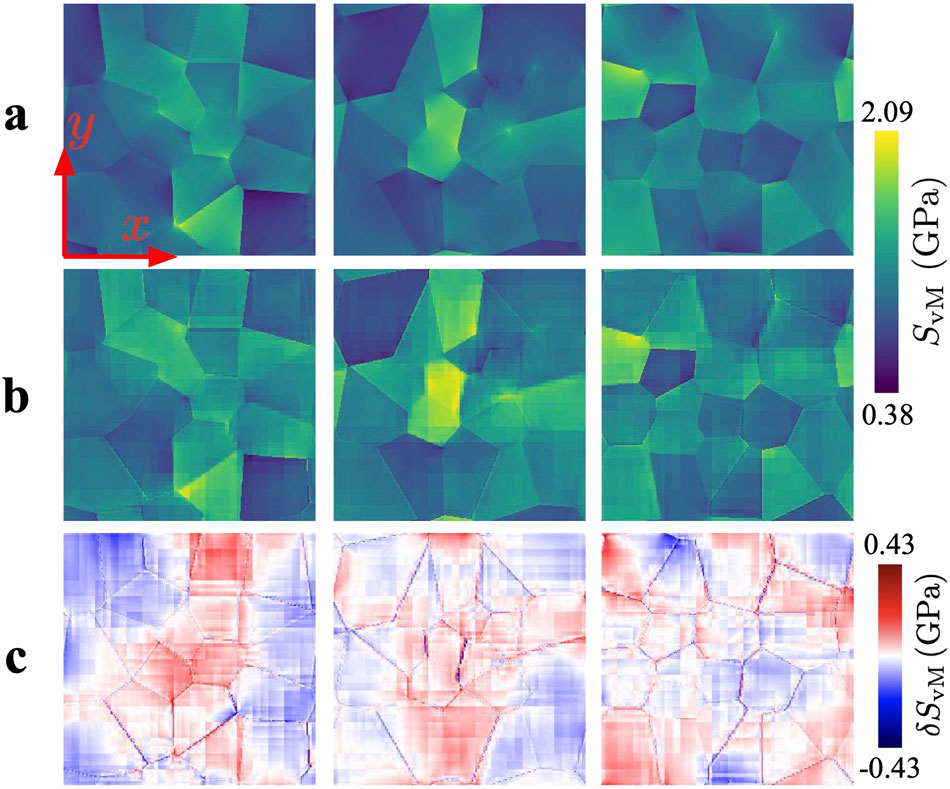
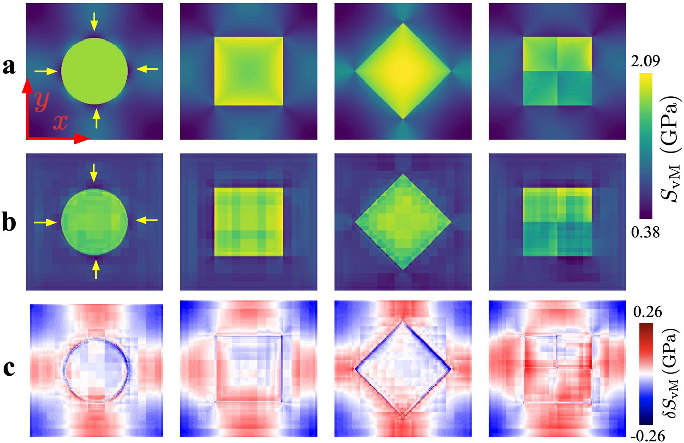
40. CNN vs 2-Point Statistics — When CNN Wins

3-D CNN architecture — voxelated microstructure → conv + pool stack → fully-connected head → effective stiffness \(C_{11}\) Mann, Andrew et al., (2022), doi:10.3389/fmats.2022.851085.

Microstructure ⇄ \(S_2\). Three voxelated two-phase RVEs (top) and their corresponding 2-point auto-correlation maps (bottom) — the classical input that the CNN replaces or complements Mann, Andrew et al., (2022), doi:10.3389/fmats.2022.851085.

CNN wins when

• Spatial features are task-specific.
• \(N \gtrsim 10^3\) specimens or simulation augmentation available.

\(S_2\) / MKS still competitive when

• \(N\) small; simulation dominates.
• Hybrid (CNN ⊕ \(S_2\)): \(R^2 > 0.96\) on stiffness regression Mann, Andrew et al., (2022), doi:10.3389/fmats.2022.851085.

Don’t pick a single winner. This slide is deliberately balanced — different methods own different regimes. That nuance is the message; tell it explicitly.

The bias-variance reframe. Low \(N\) → variance dominates → simpler input (\(S_2\)) wins. High \(N\) → bias dominates → richer input (CNN on raw pixels) wins. Same Unit-3 trade-off, different labels.

Read both figures. Left = the 3-D CNN architecture (cube → conv/pool → FC → \(C_{11}\)). Right = the same RVE expressed as \(S_2\) maps. They are different representations of the same physical microstructure — choose the one that matches your \(N\).

Pitfall to flag. “CNN beats MKS” benchmarks are usually ablations on a fixed dataset. Generalisation to new processing windows is a separate question — and often where MKS catches up.

41. Specimen Splits Revisited

Invalid protocol

1. 200 micrographs → 16 crops each → 3200 patches.
2. Random 80/20 patch split.
3. Report \(R^2 \approx 0.95\).

Reality

• Train and test share specimens → correlated rows; metric is optimistic.
• Specimen-level split on the same labels can collapse \(R^2\) to ~0.72 Sandfeld, Stefan et al., (2024).

Rule. Group ID = whatever is exchangeable at deployment.

Slow down here. This slide is the single most-violated rule in materials ML. Read both numbers aloud: \(R^2 = 0.95\) vs \(R^2 = 0.72\). Same data, same code, same algorithm — just an honest split.

The mechanism, said plainly. Crops from one specimen share thickness, etching, polishing, lighting, operator. Random shuffle puts crops from the same coupon in train and test → the model sees a near-duplicate at test time → optimistic score.

Hard rule. Group ID = whatever is exchangeable at deployment. For metallography: specimen. For AM: build. For welding: pass. Never crops or patches or frames alone.

War story I tell every year. Last summer’s project: \(R^2 = 0.95\) on patch shuffle, \(R^2 = 0.40\) on specimen split. Same code. Same student. We almost let them publish the wrong number.

Active prompt. “Tell me what your group ID is for your own current dataset.” Wait. If they can’t say it, that is the failure mode.

42. Cross-Lab Distribution Shift

• Train on microscope A: \(R^2 \approx 0.88\).
• Test on microscope B (same alloy): \(R^2 \approx 0.45\).
• CNN may latch onto contrast / vignetting / detector noise rather than grains.

Mitigations (preview Unit 6)

• Physics-aware normalisation, harmonised imaging SOPs.
• Domain randomisation / adaptation when train and deployment labs differ.
• Saliency / attention checks that the network looks where physics says it should.

Why this is harder than slide 41. Specimen split is checkable — you set the split. Cross-lab shift is invisible until it happens — the lab you trained on isn’t the lab you’ll deploy in.

The mechanism. Microscope A and microscope B differ in detector gain, vacuum, accelerating voltage, etching protocol, operator habits. The CNN may latch onto any of these proxies for class identity, and the proxies don’t transfer.

The diagnostic toolkit. Saliency maps (Grad-CAM, attention) — does the network look where physics says it should? If it focuses on the scale bar, vignetting, or the corner of the frame, you have a hidden proxy. This is exactly what slide 35’s CNN-ViT was for.

Forward signpost. Unit 6 covers transfer learning + domain adaptation in depth. Today’s takeaway: the moment your deployment lab differs from your training lab, you have a domain-shift problem — plan for it before it bites you.

43. Class Imbalance on Rare Defects

• Defect prevalence 2% → “always predict good” → 98% accuracy, 0% recall.
• Materials goal is usually high recall on the rare class.

Mitigations

• Use precision / recall / F1 or PR-AUC, not accuracy.
• Stratified specimen-level splits.
• Cost-sensitive losses; resample within train only; active labelling of hard negatives.

The trap, plainly. Defect prevalence 2% → “always predict good” classifier → 98% accuracy, zero recall. The model is statistically excellent and operationally useless.

The simple test. If your model’s accuracy is suspiciously close to \(1 - p_\text{defect}\), run the all-good baseline. Often it’s a tie — that means your model learned nothing.

Materials reframe. Most safety-critical defect tasks are recall-bounded, not accuracy-bounded. Missing a crack costs lives; flagging a non-crack costs an inspector minute. The cost asymmetry should be in the loss function, not just in the metric.

War story. Porosity detection on a real LPBF pipeline, 2% prevalence, 99% reported accuracy. We tried it on a held-out build with elevated porosity (5%) — recall was 8%. The model had memorised “predict good.” Production-disaster averted, by luck.

Active. Make them write down the metric they would use for their own project. Wait. “Anyone who said ‘accuracy’ — explain why your task is recall-insensitive.”

44. Label Noise from Upstream Segmentation

• \(\mathbf{x}\) derived from segmentation v1.3; \(y\) from pristine tensile test.
• Segmentation drift between v1.3 and v1.4 → false aleatory scatter → CNN fits artefacts.

Mitigations

• Inter-annotator / inter-version study on a subset.
• Ensemble segmentations; report label variance.
• Uncertainty-aware losses (preview Unit 12).
• Version-pin the entire upstream pipeline.

The silent failure mode. When your labels come from a model (segmentation v1.3), upgrading that model breaks all downstream predictions silently. No error, no warning — just slowly wrong numbers.

The pipeline view. Treat segmentation as part of your data, not part of your code. Pin its version like you pin numpy. Re-validate downstream models when you upgrade.

Connect. Same spirit as Unit 3’s inter-annotator-variance slide — except the “annotator” is now a numbered network version. The bias structure is identical; the cause is more insidious because it can be triggered by a routine update.

Take-home line, board-worthy. “Your \(y\)-data has noise. So does your \(\mathbf{x}\)-data. So does your labels-on-\(\mathbf{x}\) — and that one is the easiest to forget.”

45. Raw-Pixel MLP Failure → CNN Motivation

• \(1024 \times 1024\) RGB → first dense layer ≈ \(10^9\) weights.
• \(N \sim 10^2\) specimens: spurious pixel correlations dominate.
• Optimisation finds coupons, scratches, brightness gradients — not physics.

The Unit 5 punchline

• CNNs: locality + weight sharing → effective parameter count drops by orders of magnitude.
• The right inductive bias for spatial data Goodfellow, Ian et al., (2016).

Make the parameter blow-up visceral, again. \(1024^2 \times 3 \approx 3 \times 10^6\) inputs. First dense layer with 1000 hidden units = \(3 \times 10^9\) weights. With \(N=100\) specimens: that’s 30 million parameters per training example. No statistical signal can possibly survive that ratio.

What the model actually learns instead. It memorises coupon edges, brightness gradients, vignetting, the operator’s framing habits. Anything but physics.

The Unit-5 punchline. Convolution = locality + weight sharing. A 3×3 filter applied at every spatial location has 9 weights, regardless of image size. CNNs cut effective parameters by 4–5 orders of magnitude. That is why we need a lecture on CNN architectures next week.

Single cleanest motivation slide for Unit 5. Tell them to remember this argument when they walk in next Wednesday.

46. When Not to Use a CNN

Use simpler models when

• \(N\) is small (a few hundred specimens).
• Inputs are tabular composition + process.
• Regulatory / safety context demands coefficient-level audit.
• Extrapolation outside training process window is required.

Practical rule

• Always fit a serious linear / MLP / tree baseline first.
• Escalate to CNN only when grouped-CV gain survives stress tests (shift, OOD batches) Sandfeld, Stefan et al., (2024).

Note

“Use the simplest model that survives grouped CV.”

Anti-hype, on the record. CNNs are not free. Training time, deployment complexity, weak interpretability, GPU dependence, harder debugging. There is a real cost.

The simple model often wins. Tabular composition + process at \(N=200\) — a linear model often within 2% of a CNN. The linear model wins on speed, interpretability, audit, and extrapolation behaviour. The 2% you bought is rarely worth the engineering tax.

War story. A licensing hearing — black-box CNN beat linear baseline by 2% on one split. Lost the regulatory submission to “linear model with documented coefficients and conservative bounds.” The 2% wasn’t worth what it cost in trust.

Take-home, write on the board. “Use the simplest model that survives grouped CV.” Eight words. Most expensive lesson in this lecture.

§6 · Bridge & Wrap

47. The MFML Toolkit Applied Here

Forward pass / activations / training loop don’t change.

• Same \(f_\theta\), same \(J\), same backprop.
• What MFML proved: this toolkit is flexible.

What changes in materials ML

• What feeds \(\mathbf{X}\) — pixels, descriptors, \(S_2\), process vector, spectra.
• What \(y\) means — measurement chain, label noise, calibration.
• How you split — specimens, batches, instruments.
• What loss reflects deployment cost.

Closing reframe. Today’s gallery is one toolkit, sixteen problems. Forward pass, activations, backprop — none of it changed. What changed: what’s in \(\mathbf{X}\), what \(y\) means, how you split, what loss matches deployment cost.

Why this matters for paper-reading. Most materials ML papers spend 80% of their text on the architecture (the part that doesn’t change much) and 20% on the encoding/labels/splits (the part that does). Read papers in inverse proportion.

Active prompt for understanding. “If forward pass / SGD / backprop don’t change, what does materials contribute to the field?” Answer: encoding choices, label discipline, deployment context, physics constraints. That is the contribution of this whole course.

48. Looking Ahead — Unit 5 (CNNs)

Next week

• Convolution = locality + weight sharing.
• Architectures: VGG, ResNet, U-Net, ViT.
• Where each architecture fits a materials task.

Carry forward from today

• Specimen splits, normalisation, shift awareness.
• CNNs multiply debugging surface — they don’t remove obligations Goodfellow, Ian et al., (2016).

Beyond Unit 5

• Unit 6: transfer learning + domain shift.
• Unit 12: uncertainty quantification.

Tease the architecture. “Next week I’ll show you what convolution actually computes — and why a 3×3 filter beats a fully-connected layer with \(10^9\) parameters. Hint: it’s the same idea as the FFT, but learned.”

Curriculum map. Unit 5 = CNN architectures (VGG/ResNet/U-Net/ViT, what fits where). Unit 6 = transfer learning + domain shift. Unit 12 = uncertainty quantification. Today is the appetizer; the main courses are coming.

The non-negotiable carry-over. CNNs don’t relieve the obligations from §5. They add to the debugging surface — saliency maps, augmentation policy, batch-size effects. Not less work; more.

Time-permitting demo. If 2 minutes remain, show a Grad-CAM saliency failure — network attends to the scale bar instead of the grain structure. Lands the §5 lessons one last time.

49. Reading + Exercises

Reading

• Sandfeld 2024 — Ch. 17 (NN), microstructure / 2-point statistics chapters Sandfeld, Stefan et al., (2024).
• McClarren 2021 — Ch. 5 (feed-forward nets) McClarren, Ryan G., (2021).
• Neuer 2024 — Ch. 4 (supervised workflow) Neuer, Michael et al., (2024).
• Goodfellow 2016 — Ch. 9 (CNN motivation, optional) Goodfellow, Ian et al., (2016).
• Holm 2020 — single-paper survey of the field Holm, Elizabeth A. et al., (2020), doi:10.1007/s11661-020-06008-4.

Exercises

1. Reproduce Azimi-style classification on UHCS micrographs (NIST public). Compare a hand-crafted feature pipeline against a small CNN.
2. Compute binned \(S_2\) on a binary microstructure set; train an MLP on \(S_2\) and a small CNN on raw images; compare grouped-CV scores.
3. Repeat (2) with deliberate patch-level splitting; quantify how much \(R^2\) inflates vs the specimen-level baseline.

Sell the exercises. Exercise 1 reproduces today’s hero result on real public data — confidence-builder. Exercise 2 is the encoding decision rule made hands-on — calibrates intuition. Exercise 3 is the pitfall of slide 41, experienced — none of them will forget patch-vs-specimen splits after running it.

Recommended order. Exercise 3 first, exercise 2 next. The pitfall lesson (3) is the most pedagogically efficient hour of the whole semester — 20 lines of sklearn, lifelong calibration of intuition.

Reading priority. Holm 2020 first (zero math, broad map). Sandfeld Ch 17 second (textbook depth). Goodfellow Ch 9 only if they want CNN motivation in detail before next week.

Open the floor. “Stop me here for any question on §3 or §4 that I rushed past.” Last chance before takeaways.

50. Key Takeaways

• Hand-crafted metrics — interpretable, standardised, lossy by construction.

• \(S_2\) / MKS / eigen-modes — principled middle ground between scalars and pixels.

• Sixteen real applications across SEM, EBSD, TEM, XRD, X-ray CT, AM cameras, weld radiographs, RVE simulators — same convolutional toolkit, different encodings and heads.

• Representation > metric when data and SOPs allow Sandfeld, Stefan et al., (2024).

• CNNs are the right inductive bias for spatial / spectral signals — Unit 5 next Goodfellow, Ian et al., (2016).

• Specimen splits, lab shift, imbalance, segmentation noise — still your responsibility, no matter how deep the network.

Pace the fragments deliberately. One per ~5 seconds. Don’t read them — the slide does that. Add a single sentence of colour to each: a story, a number, a callback to a case study.

Land the closing line. “CNNs are not magic. They are the right inductive bias when data, splits, and metrics are honest. Honest is on you.” Pause. Don’t fill the silence.

Final cue. “Questions go to me at the door, by email, or in next week’s office hour. Thanks.” End.

Continue

• ← Previous: Unit 03 — Data quality, labels, and leakage
• → Next: Unit 05 — Unsupervised methods for materials — clustering & autoencoders
• All courses

References

Materials data science, Stefan Sandfeld & others

Advanced steel microstructural classification by deep learning methods, Scientific Reports, Seyed Majid Azimi, Dominik Britz, Michael Engstler, Mario Fritz, & Frank Mücklich https://doi.org/10.1038/s41598-018-20037-5

Overview: Computer vision and machine learning for microstructural characterization and analysis, Metallurgical and Materials Transactions A, Elizabeth A. Holm, Ryan Cohn, Nan Gao, Andrew R. Kitahara, Thomas P. Matson, Bo Lei, & Srujana Rao Yarasi https://doi.org/10.1007/s11661-020-06008-4

Machine learning for engineers: Introduction to physics-informed, explainable learning methods for AI in engineering applications, Michael Neuer & others

Machine learning for engineers: Using data to solve problems for physical systems, Ryan G. McClarren

Exploring the microstructure manifold: Image texture representations applied to ultrahigh carbon steel microstructures, Acta Materialia, Brian L. DeCost, Toby Francis, & Elizabeth A. Holm https://doi.org/10.1016/j.actamat.2017.05.014

High throughput quantitative metallography for complex microstructures using deep learning: A case study in ultrahigh carbon steel, Microscopy and Microanalysis, Brian L. DeCost, Bo Lei, Toby Francis, & Elizabeth A. Holm https://doi.org/10.1017/S1431927618015635

Deep learning for automated phase segmentation in EBSD maps. A case study in dual phase steel microstructures, Materials Characterization, T. Martinez Ostormujof, R. R. P. Purushottam Raj Purohit, S. Breumier, N. Gey, M. Salib, & L. Germain https://doi.org/10.1016/j.matchar.2021.111638

A deep learning approach for complex microstructure inference, Nature Communications, Ali Riza Durmaz, Martin Müller, Bo Lei, Akhil Thomas, Dominik Britz, Elizabeth A. Holm, Chris Eberl, Frank Mücklich, & Peter Gumbsch https://doi.org/10.1038/s41467-021-26565-5

Deep learning of crystalline defects from TEM images: A solution for the problem of “never enough training data”, Machine Learning: Science and Technology, Kishan Govind, Daniela Oliveros, Antonin Dlouhy, Marc Legros, & Stefan Sandfeld https://doi.org/10.1088/2632-2153/ad1a4e

Deep learning for semantic segmentation of defects in advanced STEM images of steels, Scientific Reports, Graham Roberts, Simon Y. Haile, Rajat Sainju, Danny J. Edwards, Brian Hutchinson, & Yuanyuan Zhu https://doi.org/10.1038/s41598-019-49105-0

Deep learning approaches for mining structure-property linkages in high contrast composites from simulation datasets, Computational Materials Science, Zijiang Yang, Yuksel C. Yabansu, Reda Al-Bahrani, Wei-keng Liao, Alok N. Choudhary, Surya R. Kalidindi, & Ankit Agrawal https://doi.org/10.1016/j.commatsci.2018.05.014

Modeling structure-property relationships with convolutional neural networks: Yield surface prediction based on microstructure images, International Journal of Plasticity, Julian N. Heidenreich, Maysam B. Gorji, & Dirk Mohr https://doi.org/10.1016/j.ijplas.2022.103506

A deep-learning technique for phase identification in multiphase inorganic compounds using synthetic XRD powder patterns, Nature Communications, Jin-Woong Lee, Woon Bae Park, Jin Hee Lee, Satendra Pal Singh, & Kee-Sun Sohn https://doi.org/10.1038/s41467-019-13749-3

Deep learning-based segmentation of lithium-ion battery microstructures enhanced by artificially generated electrodes, Nature Communications, Simon Müller, Christina Sauter, Ramesh Shunmugasundaram, Nils Wenzler, Vincent De Andrade, Francesco De Carlo, Ender Konukoglu, & Vanessa Wood https://doi.org/10.1038/s41467-021-26480-9

Monitoring of the powder bed quality in metal additive manufacturing using deep transfer learning, Materials & Design, Felix Gabriel Fischer, Max Gero Zimmermann, Niklas Praetzsch, & Christian Knaak https://doi.org/10.1016/j.matdes.2022.111029

A deep learning framework for defect prediction based on thermographic in-situ monitoring in laser powder bed fusion, Journal of Intelligent Manufacturing, Simon Oster, Philipp P. Breese, Alexander Ulbricht, Gunther Mohr, & Simon J. Altenburg https://doi.org/10.1007/s10845-023-02117-0

Machine vision defect segmentation and geometric measurement for real time quality monitoring in friction stir welding, Journal of Manufacturing Systems, Naveen Loganathan, Joel Andersson, & Vivek Patel https://doi.org/10.1016/j.jmsy.2026.01.007

A misclassification-aware explainable hybrid CNN-vision transformer framework for radiographic weld inspection, Scientific Reports, Kumar Parmar, Rituraj Jain, P. T. Anitha, A. Jayanthi, Ramesh Babu Putchanuthala, Kamal Upreti, & Terefe Bayisa Ayele https://doi.org/10.1038/s41598-026-44874-x

Teaching solid mechanics to artificial intelligence—a fast solver for heterogeneous materials, npj Computational Materials, Jaber Rezaei Mianroodi, Nima H. Siboni, & Dierk Raabe https://doi.org/10.1038/s41524-021-00571-z

Development of a robust CNN model for capturing microstructure-property linkages and building property closures supporting material design, Frontiers in Materials, Andrew Mann & Surya R. Kalidindi https://doi.org/10.3389/fmats.2022.851085

Deep learning, Ian Goodfellow, Yoshua Bengio, & Aaron Courville