Machine Learning in Materials Processing & Characterization
Unit 6: Transfer Learning as Optimization

Prof. Dr. Philipp Pelz

FAU Erlangen-Nürnberg

§1 · The Small-Data Challenge

Section roadmap. We open with the hard fact that motivates the whole unit: in materials science, labeled data is scarce, no matter how many raw frames the detector spits out. The first six slides build the case quantitatively (acquisition cost, expert-hours per label) and qualitatively (overfitting on hundreds of images, high variance across microscopes). We close Part 1 with the strategy map — the three levers we will pull for the rest of the lecture: augmentation, transfer learning, and synthetic data.

Connection to MFML W6. This week’s MFML prerequisite is Optimization for Deep Learning: loss landscapes, SGD/Adam, learning-rate schedules, batch size and gradient noise. We will lean on that material heavily in §2, where fine-tuning is reframed as continued optimization on a related landscape. Today’s framing — “transfer learning as optimization” — is what makes discriminative learning rates, gradual unfreezing, and warm-up schedules fall out as direct applications of MFML W6 instead of arbitrary tricks.

01. From scratch is the exception

• Today’s question: what do we do when we have a \(10^9\)-parameter network and \(10^2\) labeled images?
• The honest answer in modern materials ML: we almost never train from scratch.
• We continue an optimization that someone else (often the ImageNet community) already did for us.
• Three levers do almost all the work:
  1. Augmentation — synthetic diversity from existing images.
  2. Transfer learning — reuse pretrained weights as a warm start.
  3. Synthetic data — generate labeled images from physics or geometry.

MFML Unit 6 prerequisite (this week): Optimization for Deep Learning.

• Loss landscapes, gradient descent, momentum.
• AdaGrad / RMSProp / Adam, per-parameter LR.
• Learning-rate schedules, warm-up, cosine annealing.
• Batch size \(\leftrightarrow\) gradient noise.

Everything in this lecture is a special case of those ideas applied to a pretrained starting point.

Framing the unit. The materials ML lifecycle almost never looks like the ImageNet textbook story. We do not train ResNet-50 on 14 M images of grains. We have at most a few hundred labeled SEMs of a specific alloy, taken on a specific microscope, by a specific student. Training a 25 M-parameter backbone from random init on that dataset is a guaranteed overfit.

The reframing in one sentence. Transfer learning is not a trick — it is the natural mode of optimization when good initial weights exist. The pretraining gives you a warm start in a basin that already encodes generic visual features (edges, textures, blobs); fine-tuning is gradient descent in the same loss-landscape geometry MFML W6 just taught, restricted to a small, well-conditioned region near that pretrained point.

Anti-pattern war story. I once reviewed a paper where the authors trained a U-Net from scratch on 80 SEMs and reported 92 % IoU on the same 80 SEMs. The held-out test on a different microscope dropped to 41 %. Switching to an ImageNet-pretrained encoder + grouped K-fold CV would have cost them an afternoon and saved them the rebuttal.

Forward links.

• §2 is the optimization-theory core (MFML W6 cross-references).
• §3 (augmentation) and §4 (transfer learning proper) are the two main practical levers.
• §5 (synthetic data) is the “infinite-label” escape hatch.
• §6 collects the recipe and validation hygiene.

Say aloud: “If you remember one thing from today: never train from scratch when somebody has already paid the optimization bill for you.”

02. The “big data” myth in materials

• Modern detectors generate terabytes of raw data per session (4D-STEM, serial-section FIB-SEM, in-situ video).
• The labeled fraction is tiny: typically \(10^{-3}\)–\(10^{-5}\) of frames.
• ImageNet labels were crowdsourced via Mechanical Turk at $0.01 / image.
• Materials labels (a grain map, a defect mask) cost PhD-hours — $$30–60 min per SEM, often more for TEM.

• Numerical reality check. A ResNet-50 expects \(\sim 10^6\) labeled images. A typical alloy-segmentation paper has \(\sim 10^2\).
• That’s four orders of magnitude of data we don’t have.
• Closing this gap naïvely by collecting more data is impossible: the bottleneck is human expertise, not detector throughput.
• We must be smart with what we have.

The asymmetry to internalize. Raw frames are nearly free; expert labels are expensive and slow. This single asymmetry drives most decisions in materials ML: which architecture, which loss, which augmentation, what to synthesize, how to validate. The unit you are watching exists because of it.

Concrete numbers to quote.

• A modern direct-detector 4D-STEM acquisition: 30–500 GB per scan; a single beamtime can yield 10+ TB.
• Hand-segmenting a single SEM of polycrystalline metal at 20 grains × 1 min per grain ≈ 20 minutes. For 100 images, that’s ~30 PhD-hours of pure annotation labour.
• Annotating a 4D-STEM diffraction-pattern dataset is even worse: the “labels” themselves often have to be inferred from physics models.

Why ML for characterization is fundamentally different from natural-image ML. ImageNet-style projects can scale labels with budget. Materials projects cannot — the labelers are the same people writing the papers. The economics force us toward TL, augmentation, and synthetic data.

Bridge. The next slide makes the cost concrete with specific characterization techniques.

03. Why materials data is scarce

Acquisition cost per labeled sample.

• Synchrotron beamtime: $10–50 k / day, allocated 6–12 months in advance.
• Aberration-corrected STEM: $1–5 k / day instrument cost.
• Sample preparation (FIB lamellae, electropolishing) takes hours.
• In situ experiments destroy the sample — you get one shot.

Expert annotation cost.

• Segmenting 100 grains in an SEM: ~1–2 hours.
• Identifying dislocation cores in HRTEM: minutes per image, ambiguous in 10–20 % of cases.
• Phase mapping in EBSD: requires Kikuchi-pattern-by-pattern review for ambiguous indexing.
• Inter-annotator agreement is often <90 % even between experts.

Two cost terms, both binding. The total cost of a labeled materials dataset is

\[\text{cost} \;=\; N \cdot (c_\text{acq} + c_\text{label})\]

with \(c_\text{acq}\) in beamtime and \(c_\text{label}\) in expert hours. Both terms are large. ImageNet-style projects work because \(c_\text{acq} \approx 0\) (scrape the web) and \(c_\text{label}\) is crowdsourced. Neither escape hatch is available to us.

Inter-annotator agreement (the awkward truth). Even when we do label data, two senior microscopists disagree on a non-trivial fraction of grain boundaries, dislocation positions, or precipitate boundaries. So our “labels” have intrinsic noise of perhaps 5–15 %. A model that fits the training set to 99 % accuracy is therefore fitting label noise — and the augmentation / TL strategies discussed today help by injecting reasonable variability that prevents over-confident memorization.

Practical guideline. Before any TL/augmentation/synthetic-data work, estimate label noise on your dataset: have two annotators relabel a 20-image subset and compute Cohen’s \(\kappa\). If \(\kappa < 0.7\), your dataset has bigger problems than model architecture.

Linkage. This sets up the next slide on the ratio of raw to labeled data.

04. Labeled vs. raw data — the gap

• A typical 4D-STEM session produces \(\sim 10^7\) diffraction patterns.
• Of those, perhaps a few hundred have ever been hand-labeled.
• A typical SEM tomography stack: \(10^3\)–\(10^4\) slices, with maybe 10 slices fully segmented.
• The unlabeled background dominates by 3–5 orders of magnitude.

Implications for the ML pipeline.

1. Use the unlabeled background: self-supervision, pretraining on raw pixels (foreshadows W11/W14).

2. Reuse other people’s labels: ImageNet, Cityscapes, BraTS — all provide pretrained weights we can fine-tune.

3. Manufacture labels: synthetic data with perfect masks (Part 5).

The three levers come from this asymmetry. Each lever attacks one side of the inequality \(|\mathcal{D}_\text{labeled}| \ll |\mathcal{D}_\text{raw}|\).

• Augmentation multiplies the labeled side using physics-respecting transformations.
• Transfer learning substitutes pretraining on a different labeled set for the missing labels here.
• Synthetic data manufactures labeled examples by running the forward model in reverse: we know the ground truth because we generated it.

Forward link. Even after applying all three, we still typically have \(\lesssim 10^4\) effective labeled training examples. That is why the optimization recipe in §2 — small steps, low LR on the backbone, no catastrophic forgetting — is non-negotiable: we cannot afford to wreck \(10^9\) pretrained parameter updates with a careless learning rate.

The big number to internalize. ImageNet had \(\sim 10^7\) labeled images and \(\sim 10^3\) classes. We have \(10^{1-3}\) labeled images and \(10^{0-1}\) classes. The total label-content gap is a factor of \(\sim 10^4\). This is why TL is essential, not optional.

05. Overfitting in the small-data regime

• Train a ResNet-50 on 100 SEM images from one microscope.
• Training loss → 0 within a few epochs.
• Validation loss diverges; test on a different microscope drops 30–50 percentage points.
• The model memorized detector artifacts (drift bands, vignetting, fixed-pattern noise) instead of microstructural features.

Bias–variance picture (from MFML).

• High-capacity model + small dataset \(\Rightarrow\) high variance.
• Tiny perturbations of the training set move the optimum across the loss landscape by huge amounts.
• The same checkpoint, retrained with a different seed, gives a different test accuracy by 5–15 percentage points.
• this is what the bias–variance trade-off looks like in practice.

Why high-capacity nets overfit faster than students expect. A ResNet-50 has \(\sim 25 \times 10^6\) parameters. With 100 training images, the parameter-to-example ratio is \(2.5 \times 10^5\) — the network can in principle memorize the training set perfectly while being completely wrong on held-out data. Modern theory (double descent, neural-tangent kernels) tells a more nuanced story, but the practical advice still holds: more parameters than examples + no regularization = overfit.

Diagnostic checklist for the lecturer to walk through.

• Train and validation loss diverge after ~10 epochs.
• Test accuracy on a different microscope is far worse than on the same one.
• Different random seeds give noticeably different test accuracies (variance dominates).
• Removing 10 % of training data drops test accuracy substantially.
• Small label flips in 1–2 % of training images change the predictions on visually similar test images.

Connection to MFML W6. The loss landscape of an overfitting model has many sharp minima with low training loss; SGD finds whichever one is closest to the random init. A pretrained init lands you in a flat minimum that is much more robust to data perturbations — that is the underlying reason TL works. We will make this precise in §2.

Anti-pattern. Increasing model capacity to “compensate” for small data makes things worse, not better. The right move is the opposite: shrink capacity (smaller backbone), or — better — share capacity with a pretrained network (TL).

06. The strategy map

Three levers, one pipeline.

1. Augmentation \(\to\) multiplies the labeled set by encoding invariances (rotations, flips, noise).

2. Transfer learning \(\to\) reuses optimization done on a larger labeled set; warm start in a flat basin.

3. Synthetic data \(\to\) manufactures labels for free using physics or geometry simulators.

Typical real-world combination:

[ImageNet pretrained backbone]
            │  (transfer)
            ▼
[fine-tune on synthetic Voronoi]
            │  (synthetic data)
            ▼
[fine-tune on 100 real SEMs]
            │  (transfer + augmentation)
            ▼
   deployable model

• Augmentation is layered onto every fine-tuning stage.
• This pipeline is the ML-PC default, not an exotic recipe.

Walk through the diagram. A modern materials-segmentation model is typically the result of a cascade of fine-tuning stages, each one narrowing the domain. ImageNet → synthetic-Voronoi → real-SEM. At each stage we re-apply the optimization-as-fine-tuning principles of §2. Each stage uses augmentation; only the intensity of augmentation changes (mild for ImageNet→Voronoi, aggressive for Voronoi→real-SEM where the domain gap is largest).

Why all three levers, not just one.

• Augmentation alone cannot create features the data never had (e.g., rare phases). It encodes invariances, not new physics.
• Transfer learning alone gives generic features but not domain-specific ones (a network pretrained on cats has never seen a grain boundary).
• Synthetic data alone has the sim-to-real gap (§5).
• The combination wins. Each lever fixes the others’ blind spots.

Forward link. §2 explains why each lever works in optimization terms. §3–§5 explain how to deploy each one. §6 binds them into a recipe and discusses validation hygiene.

Say aloud. “By the end of today you will recognize this cascade as the default pipeline, not as an exotic recipe.”

§2 · Fine-Tuning as Continued Optimization

Section purpose. This section is the technical heart of the unit and the reason we restructured Unit 6 around optimization. Every “trick” in practical transfer learning — discriminative LRs, gradual unfreezing, warm-up, cosine schedules, the Adam→SGD switch — is a direct application of MFML W6. By the end of §2 students should see fine-tuning not as a catalogue of recipes but as one continuous optimization process across two related loss landscapes.

MFML W6 cross-references the lecturer should make explicit:

• Loss-landscape geometry, Hessian, curvature, sharp vs flat minima.
• Per-parameter LR (AdaGrad, RMSProp, Adam) — the conceptual ancestor of layer-wise LR.
• Warm-up and cosine annealing as variance-reduction tools at the start and end of training.
• Batch-size \(\leftrightarrow\) gradient-noise relationship (linear-scaling rule).
• Adam’s tendency to converge to sharper minima than SGD+momentum, and the implications for generalization.

If students did not internalize MFML W6, they will not get §2. Start with the MFML W6 callback on the next slide.

07. From SGD to fine-tuning — the same machinery

Pretraining (Task A).

• Minimize \(\mathcal{L}_A(\boldsymbol{\theta}) = \mathbb{E}_{(x,y)\sim\mathcal{D}_A}\!\left[\ell(f_{\boldsymbol{\theta}}(x), y)\right]\) on a large dataset (e.g., ImageNet).
• Lots of data, lots of compute, lots of optimization steps.
• End point: \(\boldsymbol{\theta}^\star_A\) — a flat basin of \(\mathcal{L}_A\).

Fine-tuning (Task B).

• Minimize \(\mathcal{L}_B(\boldsymbol{\theta})\) on a small materials dataset starting from \(\boldsymbol{\theta}^\star_A\).
• Same SGD/Adam mechanics. Same loss-landscape ideas.
• Only the landscape and the initial point change.

The continuity claim.

\[\boldsymbol{\theta}_{t+1} = \boldsymbol{\theta}_t \;-\; \eta_t \, \mathbf{m}(\nabla \mathcal{L}_B(\boldsymbol{\theta}_t))\]

• Replace \(\mathcal{L}_A\) with \(\mathcal{L}_B\).
• Initialize at \(\boldsymbol{\theta}^\star_A\) instead of random.
• Done. That is fine-tuning.

The non-trivial part: \(\mathcal{L}_B\) is related to \(\mathcal{L}_A\) (both are image-classification-like losses), but its minimum is at a different point. Fine-tuning is the controlled walk from one minimum to the other.

The reframing in one slide. The single most important conceptual move: stop thinking of fine-tuning as a separate algorithm. It is the same SGD/Adam you already understand, applied with two changes — different loss, different starting point. Once that lands, every “trick” in TL becomes obvious.

MFML W6 callback (say aloud). “Last week you saw that SGD’s behavior depends on three things: the loss landscape (curvature), the initialization, and the schedule. In fine-tuning, the loss landscape is similar to the one you trained on (because the network’s job — classify or segment images — is similar). The initialization is excellent (flat basin). The schedule needs to be conservative (don’t undo the pretraining).”

Mathematical setup to introduce.

• Two related distributions \(\mathcal{D}_A\) (e.g., ImageNet) and \(\mathcal{D}_B\) (e.g., your SEM dataset).
• Two loss surfaces \(\mathcal{L}_A, \mathcal{L}_B\) over the same parameter space.
• Pretraining: \(\boldsymbol{\theta}^\star_A = \arg\min \mathcal{L}_A\) — but in practice we have one specific SGD trajectory’s endpoint, not the global minimum.
• Fine-tuning: starting from \(\boldsymbol{\theta}^\star_A\), take gradient steps on \(\mathcal{L}_B\).

Caveat to mention. \(\boldsymbol{\theta}^\star_A\) is not generally a minimum of \(\mathcal{L}_B\) — but if Tasks A and B are related, it is typically inside a low-loss region of \(\mathcal{L}_B\). That is the empirical observation that makes TL work.

Bridge. Next slide makes the geometry of “related loss landscape” precise, using the MFML W6 vocabulary of Hessian, curvature, basins.

08. The transfer-learning loss landscape

Pretraining lands you in a flat basin of \(\mathcal{L}_A\).

• Local Hessian \(\mathbf{H}_A = \nabla^2 \mathcal{L}_A(\boldsymbol{\theta}^\star_A)\) has small eigenvalues — flat minimum (good for generalization, MFML W6).
• Gradient noise during pretraining acts as an implicit regularizer toward flat minima.

Why the same point is good for \(\mathcal{L}_B\).

• For related tasks, \(\mathcal{L}_B\) is approximately a perturbation of \(\mathcal{L}_A\) near \(\boldsymbol{\theta}^\star_A\).
• Flat basins of \(\mathcal{L}_A\) are typically also low-loss regions of \(\mathcal{L}_B\) — features generalize.

Fine-tuning is a controlled walk in this landscape.

• We want to stay in the basin (preserve pretrained features).
• We want to descend on \(\mathcal{L}_B\) (fit the new task).
• These two goals trade off via the learning rate.
• Too large an LR \(\Rightarrow\) leave the basin \(\Rightarrow\) catastrophic forgetting (next slide).
• Too small an LR \(\Rightarrow\) never adapt \(\Rightarrow\) underfitting on Task B.

Mental model: fine-tuning = SGD with a really good prior on where the minimum is.

Hessian intuition (MFML W6 vocabulary). A pretrained checkpoint sits in a low-curvature region of \(\mathcal{L}_A\) — small Hessian eigenvalues mean the loss is roughly flat in many directions. Two consequences:

1. Robustness to parameter perturbations. A small step in any direction barely changes the loss, so the model generalizes (MFML W6: flat minima \(\to\) better test loss).
2. Robustness to loss perturbations. If we replace \(\mathcal{L}_A\) by a related \(\mathcal{L}_B\), the same flat region is approximately low-loss for \(\mathcal{L}_B\) as well. This is the geometric reason pretrained inits transfer.

A first-order expansion. Near \(\boldsymbol{\theta}^\star_A\), \(\mathcal{L}_B(\boldsymbol{\theta}) \approx \mathcal{L}_B(\boldsymbol{\theta}^\star_A) + \nabla \mathcal{L}_B(\boldsymbol{\theta}^\star_A)^\top \delta + \tfrac{1}{2}\delta^\top \mathbf{H}_B \delta\). We start fine-tuning at the linear-term-driven phase: the gradient \(\nabla \mathcal{L}_B(\boldsymbol{\theta}^\star_A)\) may be nontrivial (the new task is different), but the curvature \(\mathbf{H}_B\) is well-behaved because we are in a flat region.

Implication for LR. In a well-conditioned local region (flat landscape), SGD can take large steps without diverging — but large steps in the wrong direction still leave the basin. The right move is small LR on the backbone (stay in the basin) and large LR on the head (the head is randomly initialized; we want it to traverse the loss landscape). This sets up the discriminative-LR slide (Goodfellow et al. 2016).

Key references for the curious student. (Keskar et al. 2017) on flat vs sharp minima; (Li et al. 2018) on visualizing loss landscapes; (Neyshabur et al. 2020) on what is being transferred in transfer learning.

09. Catastrophic forgetting as an optimization issue

Symptom. Fine-tuning destroys generic features the model painstakingly learned during pretraining.

• 14 M-image-trained edge detectors \(\to\) broken in 1000 SGD steps with the wrong LR.
• Validation accuracy on Task A collapses; Task B accuracy plateaus at a low level too.
• The model is now worse than either pretrained or scratch-trained.

Mechanism. Optimization on a non-stationary loss.

• \(\mathcal{L}_B\) has a different minimum than \(\mathcal{L}_A\).
• Large LR + many steps \(\Rightarrow\) trajectory leaves the \(\mathcal{L}_A\)-basin.
• Once outside the basin, the pretrained features are no longer protected by curvature — they drift.

Cure (MFML W6 toolkit).

• Small LR on the backbone (don’t move far).
• Per-layer / per-parameter LR (next two slides).
• LR schedules with warm-up (slide 14).
• Gradual unfreezing (slide 33).

Why “catastrophic” is the right word. The features destroyed by bad fine-tuning took \(\sim 10^{18}\) FLOPs and weeks of GPU time on ImageNet. A few hundred bad SGD steps can erase them. The asymmetry between cost of acquisition and cost of destruction is what makes “small steps” the single most important rule of fine-tuning.

Optimization view (the one to write on the board). The SGD update \(\boldsymbol{\theta}_{t+1} = \boldsymbol{\theta}_t - \eta \nabla \mathcal{L}_B(\boldsymbol{\theta}_t)\) takes you toward the minimum of \(\mathcal{L}_B\). But the pretrained features are encoded by the position \(\boldsymbol{\theta}_t\) being inside the \(\mathcal{L}_A\)-basin. There is no penalty in \(\mathcal{L}_B\) for leaving that basin — so SGD will leave it freely if \(\eta\) is too large.

Two ways to phrase the fix:

1. Implicit regularization via small LR. Take small enough steps that we never leave the basin. Empirically: backbone LR \(\sim 10^{-5}\), head LR \(\sim 10^{-3}\).
2. Explicit regularization (advanced). Add a penalty \(\lambda \|\boldsymbol{\theta} - \boldsymbol{\theta}^\star_A\|^2\) — this is “elastic weight consolidation” and related continual-learning techniques. Mention but don’t go deep; we use the implicit (small LR) approach.

Anti-pattern war story. A student loaded an ImageNet-pretrained ResNet, set Adam LR to \(3 \times 10^{-3}\) “because that’s the default”, and trained for 200 epochs. Test accuracy was worse than scratch. After dropping LR to \(3 \times 10^{-5}\) and training for 30 epochs, accuracy beat scratch by 18 points. Same architecture. Same data. The LR was the algorithm.

Forward link. The next two slides give the canonical fix: discriminative learning rates by layer group.

10. Discriminative learning rates (1/2)

The MFML W6 thread. Per-parameter LRs were the central idea of AdaGrad / RMSProp / Adam:

\[\boldsymbol{\theta}^{(i)}_{t+1} = \boldsymbol{\theta}^{(i)}_t - \frac{\eta}{\sqrt{v^{(i)}_t}+\varepsilon}\,g^{(i)}_t\]

• Different parameters get different effective step sizes.
• Adam’s \(v_t\) tracks the variance of past gradients per parameter.

Layer-wise LR is the coarsened version of the same idea.

• Group parameters by layer (or layer group).
• Hand-set LRs per group based on what we know about the role of each layer.

Three-group recipe (the standard).

Group	Role	LR
Early backbone	Generic edges, blobs	\(10^{-5}\)
Late backbone	Mid-level textures	\(10^{-4}\)
Head (new)	Task-specific	\(10^{-3}\)

Why the 10× steps? Backbone is almost right (small adjustments). Head is random (large adjustments needed). Mid layers interpolate.

Name to know. This is “discriminative fine-tuning” (Howard and Ruder 2018), originally proposed for ULMFiT in NLP and now the default recipe for fine-tuning everywhere.

Conceptual bridge from MFML W6. Adam already does per-parameter LR adaptation, automatically, based on gradient statistics. So why hand-set per-layer LRs? Two reasons:

1. Adam’s \(v_t\) is local in time. It does not know that a parameter came from pretraining. It treats every parameter as if its history started at fine-tuning step 0. We have prior knowledge (this layer is an ImageNet-trained edge detector) that Adam cannot exploit.
2. Coarse-graining by layer is robust. Per-parameter LRs are noisy on small datasets; per-layer averages give well-behaved updates without the variance.

Connection to optimal LR theory. For a quadratic loss \(\frac{1}{2}\boldsymbol{\theta}^\top \mathbf{H} \boldsymbol{\theta}\), the optimal step size is \(1/\lambda_\text{max}(\mathbf{H})\). If different blocks of the Hessian have very different eigenvalue scales (which they do across layers — the Hessian is highly non-uniform per layer), then a single LR is suboptimal: it must be set by the largest eigenvalue, which slows down everything else. Block-wise LRs solve this exactly.

Empirical rule of thumb. Set head LR by trial-and-error on a small holdout (typically \(10^{-3}\)–\(10^{-4}\) for Adam, \(10^{-2}\) for SGD+momentum). Then divide by 10 per layer group going deeper into the backbone.

Citation. ULMFiT (Howard and Ruder 2018) is the original paper.

Forward link. Next slide: the implementation in PyTorch and a practical concrete example.

11. Discriminative learning rates (2/2) — implementation

PyTorch one-liner.

optimizer = torch.optim.AdamW([
    {"params": model.early_backbone.parameters(),
     "lr": 1e-5},
    {"params": model.late_backbone.parameters(),
     "lr": 1e-4},
    {"params": model.head.parameters(),
     "lr": 1e-3},
], weight_decay=1e-2)

• Each params group can have its own LR, weight decay, and even its own schedule.

Why this works pedagogically.

• Early-backbone features (Gabor-like edge detectors) are the same for cats, cars, and grain boundaries. Tiny LR keeps them in place.
• Late-backbone features (object parts) need some adaptation: a “wheel” detector becomes a “precipitate” detector with mild updates.
• Head is randomly initialized: it must travel a long distance in parameter space, so it gets the largest LR.

Optimization-theoretic sanity check. The total effective update is

\[\|\Delta\boldsymbol{\theta}\| \approx \eta \cdot \|\nabla \mathcal{L}_B\|\]

per step per group. Backbone step is \(10^{-2} \times\) head step.

Live-coding cue. Many students have only ever instantiated a single-LR optimizer (Adam(model.parameters(), lr=1e-3)). Show them the parameter-groups syntax above; emphasize that the same PyTorch optimizer class supports per-group LRs without any custom code.

How to choose group boundaries. Two strategies:

1. Coarse, robust. Just three groups: head, last block of backbone, everything earlier. Works for ResNet, ViT, U-Net.
2. Fine, ULMFiT-style. One group per “stage” of the backbone (e.g., stage1, stage2, stage3, stage4 of ResNet); LRs in geometric progression. Slightly better but more hyperparameters.

I recommend students start with the 3-group recipe and only add more groups if they have a clear reason.

Common mistake. Students often forget to include weight_decay in each group. AdamW’s default decay is sometimes too aggressive for fine-tuning; halve it as a starting point.

Connection to MFML W6 schedules. Each group can have its own LR schedule too. Common pattern: warm-up applied to all groups, but with the head’s warm-up over fewer steps (since the head needs to converge first to avoid “leaking” bad gradients into the backbone — see slide 14).

Bridge. Next slide: when to use Adam vs SGD+momentum during fine-tuning.

12. Adam vs SGD+momentum for fine-tuning

Adam (the default first choice).

• Per-parameter adaptive LR \(\Rightarrow\) robust to small/noisy datasets.
• Fast convergence in the first ~10 epochs.
• Forgiving of misspecified base LR (the \(v_t\) term self-corrects).

Caveat (MFML W6). Adam tends to converge to sharper minima than SGD+momentum, which can cost generalization on small datasets.

SGD + momentum (for the final tightening).

• Slower convergence, but the noise structure prefers flatter minima.
• Better test-set performance, especially on small datasets (Wilson et al. 2017).

Practical workflow.

1. Phase 1 (10–30 epochs): AdamW, discriminative LRs, cosine schedule.
2. Phase 2 (5–10 epochs): switch to SGD+momentum, smaller LR, no decay.
3. Final checkpoint = best validation loss across both phases.

The “switching trick” — why it works. Adam’s adaptive LR makes early optimization fast and robust, but its update direction is biased away from the geometric mean of the gradients (it normalizes per-parameter, which distorts the natural gradient). SGD+momentum, with a fixed LR, finds flatter minima — but it is harder to tune from scratch on small data. Combining both gets you Adam’s robustness early and SGD’s generalization late.

MFML W6 callback. Last week we discussed how SGD’s noise covariance is anisotropic and approximately matches the Hessian — this implicit preconditioning biases SGD toward flat minima (a deep result; see (Mandt et al. 2017)). Adam’s noise covariance is approximately isotropic in the rescaled space, which removes this implicit regularization. Hence Adam → sharper minima → worse generalization on small data.

When to skip the switch. If you only have time for one phase, stay with AdamW. The switch typically buys you 1–3 percentage points; not always worth the extra hyperparameters.

Specific defaults that work.

• AdamW: head LR \(10^{-3}\), betas (0.9, 0.999), wd 0.01.
• SGD+momentum (final phase): LR \(10^{-4}\), momentum 0.9, no Nesterov, no weight decay.

Citation note. See (Wilson et al. 2017) for the small-data generalization claim. The reference textbook for these claims is (Goodfellow et al. 2016) Ch. 8 (“Optimization for Training Deep Models”).

Bridge. Next slide: optimizer state as a memory bottleneck — and the Lion optimizer as a halved-state alternative to AdamW.

13. Optimizer state is the memory bottleneck — Lion halves it

AdamW: two extra tensors per parameter.

• Running mean \(m_t\) and running variance \(v_t\) are stored in fp32 alongside the (often fp16/bf16) weights.
• Per-parameter memory: ~3× the parameter tensor itself.
• For a 100 M-parameter backbone in mixed precision, AdamW state alone is ~0.8 GB — meaningful on an 11 GB 1080Ti shared with activations.

Lion: one extra tensor per parameter.

• Stores only the momentum buffer \(m_t\); uses the sign of the running mean for the update — no second moment.
• Per-parameter memory: ~2× the parameter tensor.
• Same 100 M backbone: ~0.4 GB of optimizer state. Half the bottleneck.

Practical takeaway (Chen et al. 2023 (Chen et al. 2023)).

• Update rule: \[x_{t+1} = x_t - \eta \, \mathrm{sign}\!\big(\beta_1 m_t + (1-\beta_1)\, g_t\big)\]
• Matches (or beats) AdamW validation loss on vision backbones — discovered by symbolic program search over optimizer space.
• LR is 3–10× smaller than the AdamW LR you would have used; weight decay 3–10× larger.

Anti-pattern. Dropping Lion in with the AdamW learning rate — it diverges immediately. The sign-update has constant magnitude, so the LR controls the step size directly.

Why a sign-based optimizer is feasible. Most of AdamW’s job is to normalize the per-parameter gradient by \(\sqrt{v_t}\) — turning a noisy multi-magnitude gradient into a roughly unit-scale update. The sign function is the limit of this normalization: \(\mathrm{sign}(g)\) gives a unit-magnitude update along the gradient direction. For vision networks the loss landscape geometry is friendly enough — gradients across parameters live on similar scales after BatchNorm/LayerNorm — that this brutal normalization works. (For LLMs, where gradient scales across layers can span orders of magnitude, AdamW’s adaptive denominator is harder to replace.)

The 1080Ti budget, made concrete. Take a ResNet-50 backbone (~25 M params, fp16) plus an FPN + segmentation head (~5 M):

• Weights (fp16): 60 MB.
• Activations at batch 16, \(512\times 512\): ~2.5 GB (mixed precision).
• AdamW state (fp32 \(m_t\) and \(v_t\)): ~240 MB.
• Lion state (fp32 \(m_t\) only): ~120 MB.

The 120 MB difference may sound small at 25 M params, but jumps to 800 MB savings at 200 M params — exactly the threshold where modern backbones (DINOv2-base, ConvNeXt-large) start to fit only with the memory savings.

Connection to MFML W6. Last week we showed SGD+momentum and Adam as two points on a “how aggressively do we adapt per-parameter?” axis. Lion sits at the most-aggressive end: full sign-normalization. The MFML W6 flat-minima argument still applies — Lion finds slightly flatter minima than AdamW on vision tasks (Chen et al. report comparable or better test accuracy on ViT/ConvNeXt despite the cruder updates).

Anticipated student question. “Why not just use SGD+momentum if we care about memory?” Two reasons. (1) SGD+momentum is even more LR-sensitive on small data; the per-parameter sign of Lion gives back some of the robustness that adaptive methods provided. (2) Lion is the new sweet spot — Adam-like behavior at SGD-like memory cost. SGD+momentum remains valid for the Phase-2 tightening on slide 12.

Bridge. Next slide: warm-up and cosine schedules — the LR-schedule content from MFML W6 specialized to fine-tuning.

14. Warm-up and cosine schedules

The fine-tuning warm-up problem.

• The head is randomly initialized at step 0.
• Early gradients \(\nabla_\theta \mathcal{L}_B\) from the random head are huge and noisy.
• These large gradients backpropagate into the pretrained backbone.
• Result: the first few hundred steps can wreck pretraining.

Fix: linear warm-up.

\[\eta_t = \eta_\text{max} \cdot \min(1, t / T_\text{warm})\]

• Ramp LR from 0 to \(\eta_\text{max}\) over \(T_\text{warm} \approx 500\) steps.
• Gives the head time to “settle” before large updates reach the backbone.

Cosine annealing for the long tail.

\[\eta_t = \eta_\text{max} \cdot \tfrac{1}{2}\!\left(1 + \cos\!\frac{\pi t}{T}\right)\]

• Smoothly decays LR to (near) zero over \(T\) total steps.
• Final epochs run with very small LR \(\Rightarrow\) refine within the basin.
• Beats step-decay schedules empirically; matches MFML W6 derivation (geometric averaging of stochastic noise).

Combined schedule. Warm-up for first ~5 % of steps, cosine decay for the rest. This is the de-facto standard for fine-tuning.

Why warm-up, in optimization terms. At step 0 with a random head, the loss gradient is dominated by the head — the random head produces huge errors. With a large LR, those errors backpropagate as large updates to the backbone, which is exactly what we are trying to avoid. Warm-up gives the head a chance to learn approximately-correct outputs (from near-zero LR steps) before the LR rises to its full value and the updates can do real damage.

Geometric intuition for cosine. Compared to step decay (drop LR by 10× at fixed epochs), cosine annealing is smoother — no sudden gradient discontinuities — and empirically finds slightly flatter minima (Loshchilov and Hutter 2017). The cosine shape matches the expected \(1/\sqrt{t}\) decay of stochastic gradient noise’s optimal schedule, scaled to a finite horizon.

MFML W6 callback. Last week’s slide on optimal LR schedules showed that for convex stochastic optimization, \(\eta_t \propto 1/\sqrt{t}\) is optimal; for non-convex deep learning the optimal is empirical, but cosine works well across architectures and tasks. The conceptual idea — decrease LR as we approach a minimum — is the same.

Practical numbers for fine-tuning.

• \(\eta_\text{max}\) for the head: \(10^{-3}\) (Adam) or \(10^{-2}\) (SGD+momentum).
• Warm-up steps: 500–1000 (or first epoch).
• Cosine decay over the full training horizon.
• Optionally: warm restart every \(T/4\) epochs (SGDR (Loshchilov and Hutter 2017)) — useful for very small datasets where a single descent gets stuck.

Anti-pattern. Skipping warm-up and using “the default LR” for a randomly initialized head is the fastest way to undo a pretraining.

15. Batch size and gradient noise revisited

MFML W6 result. The SGD update is

\[\boldsymbol{\theta}_{t+1} = \boldsymbol{\theta}_t - \eta \, \hat{g}_t\]

where \(\hat{g}_t\) is a stochastic gradient with variance \(\sigma^2 / B\) (B = batch size).

• Smaller batches \(\Rightarrow\) noisier gradients \(\Rightarrow\) implicit regularization toward flat minima.
• Larger batches \(\Rightarrow\) smoother gradients \(\Rightarrow\) converge to sharper minima (faster but generalize less).

Implications for fine-tuning.

• Small datasets \(\Rightarrow\) small batches anyway (memory + dataset size).
• Small batches help: they regularize the optimizer toward flat minima — exactly what we want to preserve pretrained features.
• Linear-scaling rule. If you halve the batch, halve the LR (and vice versa). Keeps the update size \(\eta \, \hat{g}\) comparable.
• For fine-tuning: \(B = 8\)–\(32\) is typical and often better than \(B = 256\).

The batch-size \(\leftrightarrow\) LR coupling, derived (board work). The expected SGD update over one epoch is

\[\Delta \boldsymbol{\theta}_\text{epoch} = -\eta \sum_{t} \hat{g}_t\]

If we double the batch size, each \(\hat{g}_t\) is half as noisy, but we take half as many steps per epoch. To keep the expected progress per epoch the same, we must double \(\eta\). This is the linear-scaling rule (Goyal et al. 2017). It works up to a “critical batch size” beyond which larger batches stop helping (McCandlish et al. 2018).

For fine-tuning specifically. We want the noise. Small-batch SGD with appropriately-scaled LR is the default; the only reason to go big- batch is if your accelerator has memory to burn and you can use the linear-scaling rule confidently.

Anti-pattern: tiny batch + Adam + default LR. Adam’s \(v_t\) underestimates gradient variance for very small batches in early training, leading to unstable updates. Either warm up Adam carefully (slide 14) or use SGD+ momentum where the noise structure is clearer.

Memory-saving tricks (mention briefly). Gradient accumulation (simulate larger effective batch with smaller per-step memory) keeps the update structure of a large batch while fitting on a small GPU. Useful for tuning ViT-Large on a single 24 GB card.

Bridge. Next slide synthesizes Slides 7–14 into a single recipe.

16. From MFML optimization theory to the TL recipe

The five MFML W6 lessons, applied to TL.

1. Warm start in a flat basin — pretraining (slide 8).

2. Per-layer LR — discriminative fine-tuning (slides 10–11).

3. Schedules + warm-up — preserve pretraining (slide 14).

4. Adam → SGD+momentum — speed first, generalization last (slide 12).

5. Small batches — implicit flat-minimum regularizer (slide 15).

Synthesis.

Fine-tuning is continued optimization in a related loss landscape, starting from a flat basin, using per-layer learning rates with warm-up and cosine annealing, transitioning from Adam to SGD+momentum for the final tightening.

• Every term in this sentence is a direct application of MFML W6.
• This recipe drives all of Parts 4–6.
• The rest of the lecture is applications of these five lessons.

The transition slide. This is the explicit bridge from optimization theory (MFML W6) to applied transfer learning (the rest of Unit 6). Read the boxed quote aloud — it is the take-home for §2 and the conceptual spine for §§3–6.

Pedagogical move to make. Ask the class: “Of these five lessons, which one would surprise you most if it weren’t true?” The answer most students should converge on is #1 (warm start). The other four are consequences of #1: if we believed the loss surface was rough or that pretraining was useless, none of the recipes around it would matter. The point of §2 has been to convince students that #1 is well-founded geometrically (flat basins, related landscapes), so #2–#5 are then the natural toolkit.

Forward outline.

• §3: data augmentation (orthogonal lever — applies during fine-tuning).
• §4: transfer learning protocols (feature extraction, fine-tuning, gradual unfreezing) — direct applications of §2.
• §5: synthetic data — combines with §2 and §3.
• §6: practical recipe + validation hygiene.

Anti-pattern to call out. Some students will encounter “advanced TL methods” — adapter modules, LoRA, prompt tuning, prefix tuning. All of those are parameter-efficient variants of fine-tuning that respect the same five MFML W6 lessons. They deserve mention later in the unit (W11/W14 material), but the foundational recipe is what’s on this slide.

Say aloud: “If you remember nothing else from §2: pretraining is a warm start, fine-tuning is the same SGD/Adam you already know, and the only extra ingredient is per-layer LR schedules to preserve what pretraining bought you.”

§3 · Data Augmentation

Section purpose. Augmentation is the orthogonal lever to transfer learning: it doesn’t reuse weights, it expands the effective training set. Within the optimization picture of §2, augmentation acts on the loss surface, smoothing it by averaging over physically-equivalent inputs. Done right, it encodes invariances we know the model should respect (rotation invariance for textures, brightness invariance for detector-setting variation). Done wrong, it injects label noise (rotating a textured material that has a preferred orientation) or causes data leakage (an image and its augmented copy across train/test).

Sandfeld 19.2.5 is the canonical reference for this section.

17. Augmentation — artificially expanding the dataset

“Reusing existing images by applying transformations.” (Sandfeld et al. 2024)

• Each training image \(x\) becomes a family \(\{T_\alpha x : \alpha\}\).
• Network sees a much richer effective training set \(\tilde{\mathcal{D}} = \{(T_\alpha x_i, y_i) : i, \alpha\}\).
• The labels are unchanged if \(T_\alpha\) respects the task’s invariances.

Optimization view. Augmentation modifies the loss:

\[\mathcal{L}_\text{aug}(\boldsymbol{\theta}) = \mathbb{E}_{\alpha,(x,y)}\!\left[\ell(f_{\boldsymbol{\theta}}(T_\alpha x), y)\right]\]

• Smoother surface (averaging over \(\alpha\)).
• Implicit regularization toward \(T_\alpha\)-invariant predictors.
• Acts as a Bayesian prior: “the answer should not depend on \(T_\alpha\) when \(T_\alpha\) encodes a physical symmetry.”

Augmentation as Bayesian prior. The full Bayesian view: the augmentation distribution \(p(\alpha)\) is a prior on which transformations the world might apply between training and deployment. Marginalizing the likelihood over this prior is exactly the augmented loss above. Hence augmentation = priors that you can encode at training time without changing the model architecture.

The invariance question to ask first. What transformations leave the label unchanged?

• Random crop: only if the object/feature of interest is fully contained in every crop.
• Rotation: only if the material has no preferred orientation (isotropic texture).
• Brightness: yes, if the model should be detector-setting-invariant.
• Horizontal flip: yes for most natural images and many materials, but not for images with handedness (e.g., chiral structures).

Connection to equivariant networks (forward link, W13/W14). Instead of augmenting with rotations, you can build a network that is architecturally rotation-equivariant (e.g., E(2)-equivariant CNNs). That moves the invariance from data to architecture and is more sample-efficient. But it requires specialized libraries; augmentation is the simple, universal alternative.

Bridge. The next slides walk through specific transformation families.

18. Geometric transformations

Standard kit.

• Horizontal / vertical flips.
• 90° rotations (cheap; lossless on grid).
• Arbitrary-angle rotations (require resampling).
• Scaling / random resized crop.
• Random crops (standard for ResNet training).
• Affine warps, perspective warps.

For microstructures.

• “Up” is usually arbitrary \(\Rightarrow\) rotation invariance is physically natural.
• 90° rotations + flips are the safest default.
• Arbitrary-angle rotation works for isotropic materials; pad with reflection or wrap to avoid black corners.

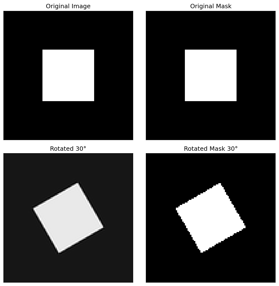
Sample augmentations applied to a microstructure image. Each row shows different rotations and flips of the same input.

Implementation pitfalls to call out.

1. Pixel-grid alignment. Arbitrary-angle rotation of integer-pixel grids requires resampling (bilinear, bicubic) — this introduces interpolation artifacts that the network can learn as “rotated” markers. Mitigation: use only 90°-multiple rotations when possible.
2. Edge effects. Rotation produces black corners. Reflective or wrap padding is preferable to zero padding; otherwise the network learns “black corner = was rotated.”
3. Random crops. Standard for ResNet training (ImageNet uses random resized crop); but for materials with a feature near the boundary of the image, random crops can chop off the very thing you want to detect.
4. Augmentation should match deployment. If your test images are \(1024\times 1024\) but you train on \(224\times 224\) random crops, you create a train-test discrepancy. Either crop to the same size at test or use sliding-window inference.

Microstructures are usually rotation-invariant, so 90°-rotation + flips is the default starting point. Combined with random crops, this typically multiplies the effective dataset by 16–64×.

Bridge. Next slide makes the rotation-invariance discussion physical: when does augmentation violate physics?

19. When transformations are “physically illegal”

The rule. \(T_\alpha\) must preserve the label.

Examples where rotation breaks the label:

• Textured materials with preferred orientation (rolled metals, drawn fibers, columnar grains).
• Imaging modalities with directional shadows (BSE detectors at oblique incidence, secondary-electron contrast).
• Crystallographic-orientation maps (rotating the image rotates the crystal frame, changing every Euler angle in the label).

Examples where flips break the label:

• Chiral structures (helical nanostructures — see (Liu et al. 2020)).
• Polarized-light micrographs (handedness matters).
• Electron-vortex / orbital-angular-momentum images.

Rule of thumb.

If your physics changes under \(T_\alpha\), don’t augment with \(T_\alpha\).

• Test for legality: ask a domain expert “would this rotated image still have the same label?”

Why this matters in practice. I have seen papers train rotation- invariant networks on rolled-metal microstructures, then complain that the network “fails to detect rolling-direction features.” The augmentation destroyed the very feature they wanted to detect. The augmentation recipe is part of the science, not boilerplate.

Diagnostic procedure.

1. Pick 5–10 images from your training set.
2. Apply each candidate transformation \(T_\alpha\).
3. Ask the labeler: “is the label still correct?”
4. If yes for all, augment with \(T_\alpha\).
5. If even one ambiguous case, don’t.

Subtle case: brightness/contrast jitter on EBSD. Brightness changes do not affect crystal orientation, so they are safe. But some EBSD software normalizes the Kikuchi pattern before indexing, in which case brightness augmentation is a no-op and just slows training.

Subtle case: vertical flip on cross-sections. A FIB cross-section typically has gravity-defined orientation (substrate at the bottom). Vertical flip swaps top and bottom, breaking the label. But horizontal flip is fine (left-right symmetry).

The takeaway slide line: “Augmentation is a physics decision, not a software decision.”

20. Elastic transformations and cutout

Elastic deformations.

• Apply a smooth random displacement field \(\mathbf{u}(x,y)\) to the image.
• Simulates stage drift, scan distortion, mild sample strain.
• Standard in medical imaging (Ronneberger et al. 2015).
• Hyperparameters: displacement amplitude \(\alpha\), smoothness scale \(\sigma\).

Cutout / random erasing.

• Black out a random rectangle (or replace with mean intensity).
• Simulates occlusions, contamination, dead-pixel rectangles.
• Forces the network to use all spatial regions, not just one.
• Generalization of dropout to image space.

Both encode physics. Elastic = drift; cutout = detector defects / artifacts.

Elastic deformation parameters. A typical recipe (from the U-Net paper): displacement field is Gaussian noise, smoothed with a Gaussian kernel of \(\sigma = 30\) pixels, scaled by \(\alpha = 50\) pixels. The result is a “wavy” version of the input that preserves topology (no folds) but locally distorts every feature.

For microstructures specifically. Elastic deformation simulates two real artifacts:

1. Scan drift in SEM/STEM: the stage moves during acquisition; the image is locally stretched along the scan direction.
2. Sample strain in in-situ experiments: the sample physically deforms during deformation/heating cycles.

Training with elastic augmentation gives drift-robust and strain-robust predictions.

Cutout’s role. Beyond defect simulation, cutout is a regularizer: it forces the network to use distributed evidence rather than a single discriminative pixel. Useful when the training set has a few very distinctive features that the network might over-rely on.

MixUp / CutMix (mention briefly). Two more advanced augmentations combine pairs of images. MixUp interpolates pixels and labels linearly; CutMix swaps rectangular regions between images. Both work well on materials data but require classification labels (or pixel-aligned masks for segmentation). Less common in the materials literature but worth trying.

21. Intensity transformations

Standard intensity augmentations.

• Random brightness shift: \(x \to x + b\), \(b \sim U[-0.2, 0.2]\).
• Random contrast: \(x \to \mu + c(x - \mu)\), \(c \sim U[0.7, 1.3]\).
• Gamma correction: \(x \to x^\gamma\), \(\gamma \sim U[0.7, 1.3]\).
• Histogram equalization.

Why this matters in materials.

• Detector dynamic range varies by setup (gain, exposure, integration time).
• Sample preparation (polishing quality, etch time) shifts contrast levels.
• Cross-microscope deployment: the physics is the same but the intensity statistics differ.

Augmenting intensity makes the model microscope-agnostic — usually the single most useful augmentation for cross-instrument generalization.

Why intensity augmentation is critical for materials ML. Unlike natural images (where every camera maps roughly the same scene to roughly the same RGB triple), materials micrographs are quantitative measurements whose absolute intensity depends on: detector gain, acquisition time, beam current, sample tilt, surface coating, and many more knobs. Two SEMs of the same sample on different machines can have completely different intensity histograms.

If your training data comes from one microscope and your deployment from another, intensity augmentation is what bridges the gap. Without it, the model overfits to the training microscope’s intensity statistics.

Practical recipe. Apply random brightness, contrast, and gamma together with mild parameters (\(\pm 20\) % each). This is what Albumentations’ RandomBrightnessContrast does by default; you usually want to add RandomGamma to it for robustness.

Caveat: don’t break the noise model. If you’re using a Poisson NLL loss (proper for low-dose images), intensity augmentation can violate the noise statistics. In that case, augment by simulating the physical cause of intensity variation (varying dose) rather than post-hoc rescaling.

Connection to Unit 2. This is a re-application of the noise-and- sensor discussion from Unit 2: real measurements are random variables with parameter-dependent distributions. Augmentation lets us sample across that parameter range at training time so the network is robust at test time.

22. Adding “physical” noise as augmentation

Physically-motivated noise types.

• Gaussian (\(\sigma\)): electronic / read noise.
• Poisson (\(\sqrt{N}\)): counting statistics, low-dose imaging.
• Gaussian blur (\(\sigma_\text{psf}\)): defocus, scan smearing.
• Salt-and-pepper: dead/hot pixels.

Match noise type to the expected detector physics (Unit 2 callbacks).

Why this works.

• At training time the network sees clean and noisy versions of the same image with the same label.
• It learns to identify structural motifs invariant to noise.
• Equivalent to a denoising auxiliary task implicitly built into the optimization.

Especially valuable for low-dose imaging (cryo-EM, beam-sensitive samples) where deployment noise is much higher than training noise.

The dose-aware augmentation principle. If you train at high dose (SNR\(_\text{train} = 30\)) and deploy at low dose (SNR\(_\text{deploy} = 5\)), the network has never seen images at deployment SNR and will fail. Fix: augment by adding noise during training to simulate the deployment SNR, or train across a range of SNRs to be dose-robust.

Match the noise model. Adding Gaussian noise to a Poisson-noise- limited sensor is a modeling error: the network learns to denoise the wrong noise model. The principled augmentation is to scale the image to a target dose and re-sample with Poisson statistics:

img_low_dose = np.random.poisson(img_high_dose * dose_ratio) / dose_ratio

This preserves the physical noise structure.

Connection to self-supervised learning. “Add noise, predict clean” is the basis of Noise2Noise / Noise2Void / SUPPORT — a whole family of self-supervised denoisers. Augmentation can be seen as a poor man’s version of the same idea, applied as a regularizer.

Beam-damage anecdote. For beam-sensitive samples (MOFs, polymers, 2D materials), training with noise augmentation lets us deploy at lower dose — meaning less damage per usable inference. The augmentation pays off in scientific impact, not just accuracy numbers.

Bridge. Next slide: how to actually implement these in code with a modern augmentation library.

23. Augmentation libraries — Albumentations / Torchvision

Albumentations recipe (typical).

import albumentations as A

train_aug = A.Compose([
    A.HorizontalFlip(p=0.5),
    A.VerticalFlip(p=0.5),
    A.RandomRotate90(p=0.5),
    A.RandomBrightnessContrast(0.2, 0.2, p=0.5),
    A.GaussNoise(var_limit=(10, 50), p=0.3),
    A.ElasticTransform(alpha=50, sigma=5, p=0.3),
])

• All operations are stochastic (probability p).
• Same Compose handles image and mask consistently.

Torchvision v2 (newer, native PyTorch).

import torchvision.transforms.v2 as T

train_aug = T.Compose([
    T.RandomHorizontalFlip(),
    T.RandomVerticalFlip(),
    T.RandomRotation(degrees=180),
    T.ColorJitter(brightness=0.2, contrast=0.2),
    T.GaussianBlur(kernel_size=5, sigma=(0.1, 2.0)),
])

• Tightly integrated with PyTorch tensors and torch.compile.
• Fewer materials-specific transforms than Albumentations.

Library choice — practical recommendations.

• Albumentations is the de-facto standard in segmentation challenges (Kaggle, MICCAI). Strong support for masks, keypoints, bounding boxes; faster than torchvision on CPU; rich set of intensity transforms.
• Torchvision v2 is improving fast and is the path of least resistance if you live entirely in PyTorch tensors. Worse mask handling but improving.
• Kornia is a third option, GPU-native — great for batched augmentation inside a training loop on large datasets.

The mask-consistency rule. If you’re doing segmentation, the mask must be transformed identically to the image. Albumentations enforces this automatically when you pass image=img, mask=mask. Doing it manually is a recipe for silent label corruption.

Augmentation magnitude calibration. Start mild (\(\pm 10\) %) and increase until validation accuracy plateaus, then back off slightly. Overly aggressive augmentation hurts accuracy on the training distribution (you’re solving a harder problem than necessary).

A common antipattern. Computing a complex augmentation pipeline on the CPU while the GPU sits idle. Profile your data loader; if augmentation is the bottleneck, move to GPU augmentation (Kornia) or reduce the per-sample cost.

Bridge. Next slide: on-the-fly vs offline; the label-consistency rule.

24. On-the-fly vs offline; the label-consistency rule

On-the-fly (the default).

• Augment inside the data loader; every batch sees fresh randomness.
• Maximum diversity, minimum disk space.
• Bottlenecks: CPU ↔︎ GPU transfer; complex transforms.

Offline (rarely needed).

• Pre-augment to disk; train on the static expanded set.
• Faster per-step (no compute at train time).
• Worse diversity (each augmented copy seen many times).
• Use when GPU is starved and CPU augmentation is the bottleneck.

Label-consistency rule (segmentation/detection).

Whatever transformation you apply to the image, you must apply identically to the mask / boxes / keypoints.

• Rotate image \(\Rightarrow\) rotate mask.
• Crop image \(\Rightarrow\) crop mask the same way.
• Brightness on image \(\Rightarrow\) no-op on mask (intensity, not geometry).
• Use library calls that take both: aug(image=img, mask=mask).

• Forget this once and you have a silently-broken dataset.

War story. A graduate student spent two weeks debugging “why does my U-Net predict shifted boundaries?” The answer: he was rotating images in NumPy and masks in PIL, with different default interpolations and different anchor conventions. The misalignment was subpixel (so visually imperceptible) but the network learned the misalignment and predicted masks that were systematically shifted by a few pixels.

The fix: always use a single library call that handles both image and mask together (Albumentations’ Compose with image=, mask= keys).

Subtle pitfall: nearest-neighbor vs bilinear interpolation. Image should be interpolated bilinearly (smooth grayscale); mask should be interpolated nearest-neighbor (preserve discrete labels). Most libraries handle this automatically when you pass them an integer mask; double-check.

On-the-fly augmentation and reproducibility. Random augmentation makes runs non-deterministic. For paper-grade reproducibility, seed the augmentation RNG separately from the rest of the pipeline. This lets you reproduce a specific run while still being able to vary augmentation experiments.

Caching trade-off. For very expensive augmentations (3D elastic deformations on volumetric data), it sometimes makes sense to cache a small set of augmented versions per epoch, refreshing them every few epochs. A middle ground between offline and on-the-fly.

Bridge. Next slide: pitfalls and section summary.

25. Augmentation pitfalls and Part 3 summary

Pitfalls.

• Don’t augment the test set. Test must be deployment-realistic.
• Don’t let an image and its augmented copy span train/test. This is augmentation-induced leakage — common, silent, and inflates accuracy by 5–20 points (we revisit in §6).
• Don’t augment past physical legality. Rotation on rolled metals, flips on chiral structures, etc.
• Don’t break the noise model by adding the wrong noise type.

Section take-homes.

1. Augmentation is a way to encode physical invariances as a prior.

2. Always augment in fine-tuning (essentially free regularization).

3. Match augmentations to the expected deployment distribution (cross-microscope, low-dose, etc.).

4. Combine augmentation with TL — the two compound multiplicatively in data efficiency.

Augmentation-leakage worked example. Take 100 images, augment each into 10 rotated copies (1000 total), randomly split 800/200 train/test. Almost every test image now has 8 of its rotated copies in the training set. The model learns to interpolate within rotation orbits; its 95 % “test accuracy” is meaningless.

The fix: split before augmentation. Decide which 80 original images are in train and which 20 are in test, then augment only the train side. Group K-fold CV (Unit 3 callback, revisited in §6) is the formalization of this rule.

The augmentation × TL multiplicative effect. Pretraining gives a better init; augmentation gives a better effective dataset. The two are orthogonal: combining them gives roughly the product of their individual gains, not the sum. This is why the canonical materials ML recipe uses both, always.

One tip per pitfall (action items for students).

• Test set: turn off all augmentation in your validation/test data pipeline. Use a separate, deterministic transform stack.
• Leakage: enforce splitting by specimen or original image ID, not by augmented sample ID.
• Physical legality: write a 1-page “what does my domain expert say?” doc before tuning augmentation parameters.
• Noise model: prefer simulating the physical cause of variation rather than post-hoc image manipulation.

Bridge. Section 4 (Transfer Learning proper) starts now.

§4 · Transfer Learning

Section purpose. §2 gave us the optimization theory; §3 gave us the data-side lever. §4 is the workhorse practical recipe — feature extraction, fine-tuning, and gradual unfreezing — applied to canonical materials problems. Sandfeld 19.2.4 (“Learning on peas to count lentils”) is the textbook reference; the Au nanoparticle U-Net (Sandfeld 19.3.1) is the success-story case study.

Pedagogical goal. Students should leave §4 able to write the PyTorch code for any of feature-extraction, fine-tuning, or gradual- unfreezing protocols, and to choose between them based on dataset size and domain gap.

26. Concept — knowledge reuse

“Learning on peas to count lentils.” (Sandfeld et al. 2024)

• Train a model on Task A (lots of data) → reuse weights for Task B (little data).
• The hope: low-level features (edges, textures, blobs) are shared between A and B.
• The empirical fact: it works spectacularly well across natural images and many scientific imaging modalities.

Optimization view (§2 callback).

• Pretrained \(\boldsymbol{\theta}^\star_A\) sits in a flat basin of \(\mathcal{L}_A\).
• For related Task B, that basin is approximately a low-loss region of \(\mathcal{L}_B\).
• We start fine-tuning inside a good region — orders of magnitude less data needed than a cold start.

Quantitatively. ImageNet-pretrained ResNet on 100 medical/materials images typically beats scratch-trained ResNet on 10 000 images.

The ImageNet \(\to\) everything-else story. Across medical imaging, remote sensing, materials, and even some non-image modalities (audio spectrograms, geophysics), ImageNet pretraining beats scratch training by large margins. This is not because ImageNet contains examples that look like the target domain — there are no grain boundaries on ImageNet. It is because the features learned (edges, blobs, repetitive textures) are universal across imaging.

Transferability empirical hierarchy (Yosinski et al. 2014):

• Layer 1 features transfer to anything (Gabor-like edge detectors).
• Layer 2–3 features transfer to most natural-image-like tasks.
• Layer 4–5 features transfer to similar tasks (other natural images of objects).
• Final layers are task-specific and rarely transfer.

This empirical observation is the empirical foundation for the discriminative LR recipe of §2: low LR on the universal layers, high LR on the task-specific ones.

Materials-specific transfers that work well.

• ImageNet → SEM (Sandfeld 19.3.1): grain segmentation, defect detection.
• ImageNet → TEM: nanoparticle counting, atom column detection.
• ImageNet → X-ray CT: pore segmentation, fiber tracing.
• Medical (BraTS, ISIC) → microscopy: similar low-level statistics.

Materials-specific transfers that do not work well.

• Natural images → 4D-STEM diffraction patterns (totally different statistics).
• Natural images → atom-probe point clouds (3D point data, not 2D image).

The forward-pass discussion (next slide) makes this concrete via hierarchical features.

27. ImageNet pretraining and hierarchical features

ImageNet at a glance.

• 14 M images, 1000 classes (cats, cars, mushrooms…).
• Hundreds of GPU-years of optimization done by the community.
• Standard pretrained checkpoints (ResNet, ViT, ConvNeXt) downloadable from PyTorch / HuggingFace.
• None of the classes are grain boundaries — yet pretraining still helps. Why?

Hierarchical feature reuse.

• Early layers learn edges, blobs, color contrasts → universal.
• Middle layers learn parts (eyes, wheels, textures) → mostly reusable.
• Late layers learn class-specific concepts → throw away.

The trick: keep the universal early layers, replace the class-specific late ones.

• This decomposition is the basis for the backbone / head split.

Why hierarchical reuse is the right mental model. Convolutional networks (and to a different but related extent, ViTs) build features compositionally: simple features at low layers combine into more complex features at higher layers. The first-layer convolutions of any trained-on-natural-images CNN are visibly Gabor-like edge detectors — regardless of the architecture or training set.

This compositional structure is why TL works across very different top-level tasks. The compositional building blocks at the bottom are shared; the compositions at the top differ.

Empirical evidence (board work). Visualize first-layer filters of: ResNet-50 trained on ImageNet, ResNet-50 trained on cancer histology, ResNet-50 trained on satellite imagery. They look essentially identical — Gabor-like edge detectors at multiple scales and orientations. Higher layers diverge dramatically.

Forward link to ViTs. Vision Transformers do not have a strong hierarchical bias by architecture, but they learn a hierarchical structure during training. Empirically, ViT features transfer comparably to CNN features for materials tasks. The choice between ResNet vs ViT backbone is more about compute and dataset size than transfer quality.

Practical pretraining sources to mention.

• torchvision.models.resnet50(weights="DEFAULT") (ImageNet-1k).
• timm.create_model("convnext_base", pretrained=True) (large library of architectures and pretraining sets).
• HuggingFace transformers for ViT, DINOv2, SAM.
• Domain-specific: BraTS-pretrained U-Nets, MicroNet pretrained models.

Bridge. Before formalizing backbone + head: ImageNet supervised pretraining is not the only — or even the best — source of generic features for microscopy. Next slide compares modern self-supervised alternatives.

28. Modern Self-Supervised Features for Microscopy

Three backbones, one steel-defect benchmark.

On a NEU-DET-style steel surface defect classification / detection task:

• ImageNet ResNet-50 (supervised). baseline. trained for 1000-class image classification.
• DINOv2-small (self-supervised on natural images) (Oquab et al. 2024). Trained on 142 M curated natural images — no labels.
• MAE pretrained on the lab’s own micrographs (He et al. 2022).

Practical recipe.

# Off-the-shelf DINOv2 features (inference)
import torch
m = torch.hub.load(
    'facebookresearch/dinov2', 'dinov2_vits14')
m.eval()                       # frozen feature extractor

# Domain MAE pretraining
import timm
backbone = timm.create_model(
    'vit_base_patch16_224.mae', pretrained=True)
# then continue MAE pretraining on your micrographs

Two adaptation paths.

• Frozen backbone + linear/MLP head. Cheapest. Works surprisingly well with DINOv2 — that’s the selling point.

Note

1080Ti budget. DINOv2-small inference and LoRA fine-tuning fit fine. DINOv2-large full fine-tuning does not — use LoRA or stick to the frozen-features path.

Empirical pattern (not exact numbers).

• DINOv2 generic features often match or beat ImageNet supervised features on metallography — the SSL training on textured natural images is closer to micrograph statistics than ImageNet’s object-centric labels.
• MAE-on-domain-data tends to beat both once ≥10k unlabeled micrographs are available.

Why DINOv2 transfers so well to microscopy. DINOv2 is trained with self-distillation on natural images that include enormous amounts of texture and fine structure — fur, foliage, fabric, stone, lichen, water, sand. The SSL objective (image-level + patch-level invariance under augmentations) forces the network to learn texture- and edge-statistics features that are not tied to ImageNet’s object-centric labels. Those features turn out to be very close to what metallography and ceramography backbones need: oriented edges, grain texture, periodic structure, defect boundaries.

Why MAE on lab data closes the remaining gap. MAE (masked autoencoder) reconstructs the masked patches of an image from the visible ones. The pretext task forces the encoder to learn the generative statistics of the input distribution. When that input distribution is your own micrographs (SEM, optical, EBSD), the resulting features are tailored to your acquisition pipeline — detector noise, contrast distribution, magnification range. ≥10k unlabeled images is the empirical break-even where MAE-on-domain stops underperforming a well-pretrained ImageNet backbone and starts beating it.

The materials hook. Most ML-PC students have access to labeled data in the hundreds, but unlabeled micrographs in the thousands to tens of thousands — the LIMI archive, every old PhD thesis backup, the QC microscope’s daily output. MAE pretraining turns that previously-useless pile into a domain-specific backbone.

Anti-pattern to call out. Fine-tuning DINOv2-large (~1.1 B params) end-to-end on a 1080Ti. Optimizer state alone (AdamW) is ~13 GB — won’t fit. Either (a) freeze the backbone and train a linear/MLP head, (b) use LoRA, or (c) drop to DINOv2-small (~22 M).

MFML W6 pointer. The “warm start in a flat basin” argument from §2 applies more strongly to SSL features than to ImageNet supervised features — SSL pretraining converges to flatter minima (empirically; Oquab et al. 2024) because the loss is averaged over augmentation distributions, which acts as implicit regularization.

Anticipated student question. “If MAE-on-lab-data is best, why bother with DINOv2 at all?” Because you usually don’t have ≥10k micrographs at project start. DINOv2 is the strong zero-shot default; MAE-on-domain is the upgrade path once your lab’s unlabeled archive is large enough — and combining both (DINOv2 init, MAE continued pretraining on lab data) often wins outright.

Bridge. Backbone + head = the structural decomposition. Next slide formalizes it.

29. Backbone and head

Backbone.

• The bulk of the network — feature extractor.
• ResNet-50 stages, ViT transformer blocks, U-Net encoder.
• Generic. Reusable across tasks.

Head.

• The final layer(s) — classifier or decoder.
• Typically: linear classifier (classification), \(1\times 1\) conv (segmentation), MLP (regression).
• Task-specific. Replaced for every new task.

The TL workflow in two lines.

# 1. Load backbone + head from pretraining
model = resnet50(weights="DEFAULT")

# 2. Replace head for the new task
model.fc = nn.Linear(2048, num_target_classes)

• Backbone keeps pretrained weights.
• Head is randomly initialized for the new task.
• Then choose: feature-extraction or fine-tuning (next slides).

The architectural anatomy. Most modern architectures have an explicit backbone/head split:

• ResNet-50: backbone = conv1 through layer4 (~25 M params); head = avgpool + fc linear classifier (~2 M params).
• ViT-Base: backbone = patch embedding + 12 transformer blocks (~85 M); head = MLP head on the CLS token (~few M).
• U-Net: backbone = encoder; head = decoder + final \(1\times 1\) conv. Note: decoders are usually trained from scratch even when encoders are pretrained.
• DETR / Mask R-CNN: backbone (ResNet/ViT) + neck (FPN) + heads (classification, box, mask). Multi-head architectures complicate the TL recipe but the backbone/head principle still applies.

Practical PyTorch tips.

• Use nn.Linear(in_features=model.fc.in_features, ...) to avoid hardcoding 2048.
• For segmentation models from segmentation_models.pytorch, the encoder argument lets you pick any pretrained backbone.
• For timm models, model.reset_classifier(num_classes=...) does the head replacement automatically.

Common mistake. Replacing only the classifier weights but not the classifier bias, or using a pretrained head as the new head. Both lead to subtle bugs. Always reinitialize the head.

Bridge. Once we’ve split into backbone + head and replaced the head, the next decision is whether to train the backbone at all. Two choices: freeze (feature extraction) or unfreeze (fine-tuning).

30. Strategy 1 — Feature extraction

Recipe.

1. Load pretrained backbone + head.
2. Replace head for new task.
3. Freeze the backbone (param.requires_grad = False).
4. Train only the head.

Implementation (PyTorch).

for p in model.backbone.parameters():
    p.requires_grad = False

# Only head params are passed to optimizer
optimizer = AdamW(model.head.parameters(), lr=1e-3)

When to use it.

• Very small datasets (\(< 100\) labeled examples).
• Target task is very similar to pretraining.
• Limited compute / time budget.
• Need a quick baseline.

Optimization view (§2).

• Effective parameter count drops from \(\sim 25\) M (full ResNet) to \(\sim 2\) M (head only).
• Tiny parameter count \(\Rightarrow\) tiny dataset suffices to fit.
• Almost no overfitting risk.

Why feature extraction is a great default. It’s boring — the backbone never moves, so the only thing being optimized is a small linear (or MLP) head. The optimization problem is essentially convex (linear classifier on fixed features), the dataset requirement is small, and the recipe is trivially reproducible. This is what to try first on any new dataset.

Common improvement. Add a small MLP head (2–3 layers) instead of a single linear classifier. The MLP can learn task-specific feature combinations. Not always better, but worth trying when single linear underfits.

The hidden cost. Backbone features are fixed — if the natural- image features don’t suit your data (e.g., 4D-STEM diffraction patterns, APT point clouds), feature extraction can’t fix that. You need fine-tuning to adapt the features.

Diagnostic. If feature extraction gives 70 % accuracy and fine-tuning (next slide) gives 85 %, the gap is “what fine-tuning teaches the backbone about your domain.” If feature extraction equals fine-tuning, the backbone features were already perfect — common for very-similar-domain tasks.

Linear-probing protocol. A specific feature-extraction setup popular in self-supervised-learning evaluation: train only a linear classifier on top of frozen features. Used to benchmark how good the features are. Useful to know about; see SimCLR (Chen et al. 2020).

Bridge. Strategy 2 unfreezes the backbone for stronger adaptation.

31. Strategy 2 — Fine-tuning (full)

Recipe.

1. Load pretrained backbone + new head.
2. Unfreeze everything (or unfreeze gradually — slide 33).
3. Apply the full §2 recipe:
   • Discriminative LRs.
   • Warm-up + cosine schedule.
   • Adam → SGD+momentum switch.
   • Small batches.

Result. Backbone adapts to the new domain.

When to use it.

• \(\gtrsim 100\) labeled examples (rule of thumb).
• Domain gap between pretraining and target task is significant.
• You can afford the longer training time.

Optimization view.

• Effective parameter count = full network (\(\sim 10^7\)–\(10^8\)).
• Discriminative LRs (slide 10) and small steps (slide 9) keep us in the pretrained basin.
• Outperforms feature extraction on essentially every materials task with \(\geq 100\) labels.

The strategy choice in one sentence. Feature extraction if you have \(<100\) labels and similar domain; fine-tuning otherwise.

The “linear-probing then fine-tuning” pattern (Kumar et al. 2022). A useful refinement: do feature extraction for a few epochs first (head learns reasonable outputs), then unfreeze for fine-tuning. The pre-trained-head step prevents large gradients from the random head wrecking the backbone in the first few steps. This is related to warm-up (slide 14) but acts on the architecture rather than the LR.

Empirical numbers to quote. On a typical SEM segmentation problem with 200 labeled images:

• Scratch ResNet-50 U-Net: ~50 % IoU (severe overfit).
• ImageNet feature extraction: ~70 % IoU.
• Full fine-tuning with discriminative LRs: ~82 % IoU.
• Above + augmentation: ~87 % IoU.
• Above + synthetic pretraining: ~91 % IoU.

The cumulative effect of stacking the levers is dramatic; each one alone is a few points.

Pitfall. Full fine-tuning with a uniform high LR (e.g., \(10^{-3}\) on all parameters) usually performs worse than feature extraction — catastrophic forgetting (slide 9) wipes out the pretrained features. The discriminative LR recipe is what makes full fine-tuning safe.

Forward link. The next slide is a direct §2 recap applied here; slide 33 introduces gradual unfreezing.

32. Layer-wise LRs in practice (recap of §2)

The fine-tuning LR menu (typical starting point for ResNet-50 + custom head):

Layer group	LR (Adam)	LR (SGD+momentum)
Head (new)	\(10^{-3}\)	\(10^{-2}\)
Layer 4	\(10^{-4}\)	\(10^{-3}\)
Layer 3	\(10^{-4}\)	\(10^{-3}\)
Layer 2	\(10^{-5}\)	\(10^{-4}\)
Layer 1	\(10^{-5}\)	\(10^{-4}\)

Why it works.

• Head was random — needs to traverse the loss landscape.
• Layer 4 (semantic) — moderate adjustment to materials concepts.
• Layers 1–2 (Gabor-like edges) — small adjustment if any.

Combine with §2 recipe.

• Warm-up over first 5 % of steps.
• Cosine annealing for the rest.
• Small batches (\(B = 16\)–\(32\)).
• Switch to SGD+momentum for the last 20 % of steps.

Where the numbers come from. These LRs are the result of a decade of empirical practice ((Howard and Ruder 2018); HuggingFace and timm defaults; fastai defaults). They are starting points — tune \(\eta_\text{head}\) on a small validation set, then keep the 10× ratios fixed.

An LR-finder shortcut. The “LR-finder” (Smith 2017): sweep LR exponentially from \(10^{-7}\) to \(10^{-1}\) over a few hundred steps, plot loss vs LR. The optimal \(\eta_\text{head}\) is where loss decreases steepest, one decade smaller than where loss diverges. Then divide by 10 per layer group.

Two-line PyTorch idiom (recap from slide 11).

optimizer = AdamW([
    {"params": model.head.parameters(),     "lr": 1e-3},
    {"params": model.layer4.parameters(),   "lr": 1e-4},
    {"params": model.layer3.parameters(),   "lr": 1e-4},
    {"params": model.layer2.parameters(),   "lr": 1e-5},
    {"params": model.layer1.parameters(),   "lr": 1e-5},
    {"params": model.conv1.parameters(),    "lr": 1e-5},
])

MFML W6 callback. This is exactly per-parameter LR adaptation (AdaGrad/Adam) coarsened to per-layer groups. Using both Adam and discriminative LRs is intentionally redundant: Adam’s per-parameter adaptation handles fine-grained variation; discriminative LRs encode the per-layer prior we get from the backbone/head split.

Bridge. Slide 33: gradual unfreezing as an extra safety measure.

33. Gradual unfreezing

The procedure (ULMFiT-style).

1. Freeze all but head; train head to convergence (\(\sim 5\) epochs).

2. Unfreeze the last backbone block; train (\(\sim 5\) epochs).

3. Unfreeze the second-to-last block; train.

4. Continue until all layers are unfrozen.

5. Optional: final fine-tuning with the full §2 recipe.

Why it works (optimization view).

• Each phase is a small-parameter optimization in a good basin.
• The head learns first — its gradients become well-conditioned before they reach the backbone.
• Avoids catastrophic forgetting at the architecture level, not just via small LRs.

When to use it. Very small datasets, large domain gap, or when plain fine-tuning is unstable.

Why gradual unfreezing helps when discriminative LRs alone aren’t enough. Even with backbone LR \(10^{-5}\), thousands of gradient steps can drift the backbone out of the pretrained basin if those gradients are systematically biased (as they are when the head is random). Gradual unfreezing fixes this by ensuring the head is near-converged before backbone gradients ever flow.

The trade-off. Gradual unfreezing roughly doubles the training time (many short phases instead of one long one). For datasets where simple fine-tuning works, skip it. For datasets where simple fine-tuning gives unstable training (loss spikes, divergence after a few epochs), unfreezing gradually almost always rescues it.

Implementation: a callback. Most modern training libraries (PyTorch Lightning, fastai, transformers) provide a “discriminative unfreezing” callback. In raw PyTorch, you set requires_grad per layer and recreate the optimizer at each phase.

Connection to curriculum learning. Gradual unfreezing is a special case of curriculum learning: present the optimization with progressively harder problems. The head-only problem is easy; the head + last block is medium; the full network is hard. This curriculum is what keeps us in the pretrained basin.

Modern PEFT alternatives. LoRA, adapters, prefix-tuning, and prompt- tuning are parameter-efficient fine-tuning methods that train only a small subset of new parameters while keeping the backbone frozen. They are gradual unfreezing pushed to the extreme: instead of unfreezing existing weights, add a small number of new weights. Worth a mention, deeper coverage in W11/W14.

Bridge. Next slide: when does TL fail? Domain-gap considerations.

34. Domain gap — natural vs scientific images

Where natural-image features do transfer.

• Edges, blobs, repetitive textures.
• Local statistics (Gabor-like first layer).
• Multi-scale composition.
• Most practical materials-imaging tasks (SEM, BSE, optical microscopy).

Where they don’t.

• 3D coordinates / point clouds (APT) — wrong topology.
• Diffraction patterns (4D-STEM) — totally different statistics.
• Hyperspectral cubes (\(x,y,E\)) — extra spectral axis.
• Ultra-low-dose images — natural images are noise-free; need Poisson-aware pretraining or noise-augmented fine-tuning.

Diagnostic. If feature extraction performs worse than scratch training, the pretrained features actively mislead — switch backbone or pretrain on a closer source domain.

The “right backbone for the right task” heuristic.

• 2D real-space materials images \(\to\) ImageNet ResNet/ViT/ConvNeXt.
• Medical-imaging-style data \(\to\) medical-imaging pretrained (BraTS, MoCo-CXR, RadImageNet).
• Volumetric / 3D image \(\to\) MedicalNet, 3D ResNet, or train from scratch on synthetic 3D.
• 4D-STEM, hyperspectral \(\to\) usually pretrain on synthetic or self-supervise on raw data; ImageNet is a poor source.
• APT point clouds \(\to\) PointNet variants pretrained on ShapeNet.

The “natural-image bias” trap. ImageNet is biased toward photographs: 3-channel RGB, perspective distortion, natural lighting, characteristic texture statistics. If your domain breaks any of these, pretraining helps less.

Mitigations.

1. Adapt the input pipeline. Replicate single-channel grayscale to 3 channels; normalize using ImageNet’s mean/std (or your domain’s).
2. Use domain-specific pretraining. Many fields now have public pretrained models (e.g., MedicalNet, microscopy-specific weights).
3. Self-supervise on raw data. Train a SimCLR/DINO/MAE on your unlabeled raw frames; the resulting features are domain-native.
4. Mix sources. Pretrain on ImageNet + fine-tune on synthetic → fine-tune on real (cascade pretraining).

Empirical guidance. When you suspect a domain gap, run a quick comparison:

• ImageNet feature extraction vs scratch training, both with augmentation.
• If ImageNet \(\gg\) scratch, TL works.
• If ImageNet \(\sim\) scratch, you have a domain gap; consider self- supervised pretraining.
• If ImageNet \(<\) scratch (rare but real), the pretraining is harmful.

Bridge. Within the materials world there are also domain gaps — across microscopes, samples, alloys. Slide 35.

35. Cross-microscope and within-domain transfer

A more friendly TL setup.

• Pretrain on a high-end aberration-corrected TEM dataset.
• Fine-tune on a lower-end, more accessible TEM.
• Both share the same physics; only acquisition parameters differ.

Why it usually works very well.

• Tiny domain gap \(\Rightarrow\) pretrained basin is essentially the target basin.
• Small fine-tuning datasets suffice.
• Often feature extraction is enough (no full fine-tuning needed).

Generalizes:

• Synchrotron \(\to\) lab X-ray.
• One alloy system \(\to\) a related alloy system.
• One operator’s images \(\to\) another operator’s images.

The within-domain-TL workflow. The most successful materials-ML projects often do two TL stages:

1. Off-the-shelf pretraining (ImageNet) → strong generic features.
2. In-house pretraining (a previous related materials dataset) → domain-specific features.
3. Final fine-tuning on the small target dataset.

Stage 2 is what makes the difference between “decent” and “publishable” results in materials ML. If your group has any prior labeled dataset in a related domain, use it for stage 2.

Cross-microscope normalization. Different microscopes have different intensity statistics, scan parameters, detector response functions. The intensity augmentation discussed in §3 (slide 21) is exactly the right tool to bridge this gap during training, so the model is robust at deployment.

Anecdote. A group at FAU trained a defect-detection network on operator A’s images of an alloy. Deploying on operator B’s images of the same alloy on the same microscope dropped accuracy by 12 points — purely because A and B used different brightness/contrast settings. After adding intensity augmentation, the gap closed entirely. The “domain” was not the alloy or even the microscope; it was the operator’s defaults.

Foreshadowing. This is exactly the “process windows” robustness discussion of W8 — generalization across operators, tools, and process conditions.

36. Success case — Au nanoparticles U-Net

Setup. (Sandfeld et al. 2024) §19.3.1

• Task. Segment crystalline gold nanoparticles from amorphous carbon background in TEM images.
• Data. \(\sim 50\)–\(100\) labeled TEM frames.
• Model. U-Net with ImageNet-pretrained encoder (ResNet-34 backbone); decoder trained from scratch.
• Recipe. Discriminative LRs, intensity augmentation, gradual unfreezing.

Outcome.

• High-fidelity segmentation despite very limited labels.
• Model handles low-contrast TEM frames where classical thresholding fails.
• Demonstrates the complete recipe: pretraining + augmentation + discriminative fine-tuning.
• This is the canonical materials-ML success story.

Predicted nanoparticle segmentation on a held-out TEM frame using the recipe described above.

The recipe walked through, slide by slide.

• Backbone pretraining (slide 27). ImageNet-trained ResNet-34 encoder. The ~25 M parameters of the encoder come pre-loaded with edge, blob, and texture detectors — exactly what we need for nanoparticle silhouettes.
• Backbone/head split (slide 29). The U-Net decoder is the “head” here, randomly initialized.
• Strategy choice (slides 28–29). Full fine-tuning, not feature extraction — encoder needs to adapt to TEM contrast statistics.
• Discriminative LRs (slide 32). Decoder LR \(\sim 10^{-3}\), encoder LR \(\sim 10^{-4}\).
• Augmentation (§3). Intensity jitter (different microscope settings), 90° rotations + flips (orientation invariant), elastic deformations (drift-robust).
• Validation (§6). Group K-fold by sample (different particles in different folds, no leakage).

Why this is the canonical example. Every lever in the unit shows up in this single example. Sandfeld 19.3.1 is worth re-reading after the full unit for that reason.

What’s not shown but is usually present. Augmentation-aware validation splitting (slide 25); a clean held-out test set on a different microscope (§6 best practices); careful initialization of the U-Net decoder layers (e.g., Kaiming init).

Take-home. When asked “should I do TL?” the answer for any SEM/TEM/optical-image segmentation problem is essentially always yes, and the U-Net + ImageNet-encoder recipe is the default starting point.

§5 · Learning from Synthetic Data

Section purpose. When labels are truly unavailable — even with TL and augmentation — synthetic data offers an escape: simulate the microstructure, get perfect labels for free, train on synthetic, deploy on real. The optimization view: synthetic pretraining = an additional pretraining stage that lands us in a basin even closer to the materials target task than ImageNet does.

Sandfeld 19.3.2 is the textbook reference; the Voronoi grain example (Sandfeld Fig 19.11) is the canonical demonstration.

Big idea. Synthetic data closes the labeling gap, but opens a new sim-to-real gap. Closing that second gap is the technical challenge of the section.

37. The “infinite data” dream

• If we can simulate the microstructure, labels are free:
  • Voronoi tessellation \(\to\) exact grain boundaries.
  • Phase-field simulation \(\to\) exact phase masks.
  • Diffraction simulation \(\to\) exact orientation maps.
• Generate as many examples as compute allows.
• No expert annotation required.

The catch. Synthetic data is too clean.

• No detector noise, no PSF blur, no scan distortions.
• A network trained only on synthetic learns to rely on artifact-free features that don’t exist in real images.
• Test on real data \(\to\) failure.

• Closing this sim-to-real gap is the technical challenge.

The synthetic-data ladder. Three increasing levels of effort:

1. Pure geometry. Voronoi grains, random spheres for nanoparticles, procedural defects. Free, fast, but the largest sim-to-real gap.
2. Geometry + physics. Add diffraction simulations, electron-beam forward models, scintillator PSFs, shot noise. Closer to real, more compute.
3. Full forward model. Multi-slice TEM/STEM simulation, finite-element for AFM-tip-sample interaction. Realistic but expensive.

Most materials groups stop at level 1 or 2; level 3 is a research project in itself.

Why “free labels” is overhyped. The labels are free, but evaluating whether the synthetic distribution covers the real one is not. A model that’s perfect on synthetic and fails on real is worse than no model at all — it gives the user false confidence.

The right deployment workflow.

1. Generate synthetic dataset.
2. Pretrain on synthetic.
3. Fine-tune on a small real labeled set — even 10–20 real images make a huge difference.
4. Validate on a held-out real test set.

This pretraining-on-synthetic + fine-tuning-on-real is the modern best practice. The next slides walk through the components.

Bridge. Slide 38: the simplest synthetic-data generator — Voronoi tessellations.

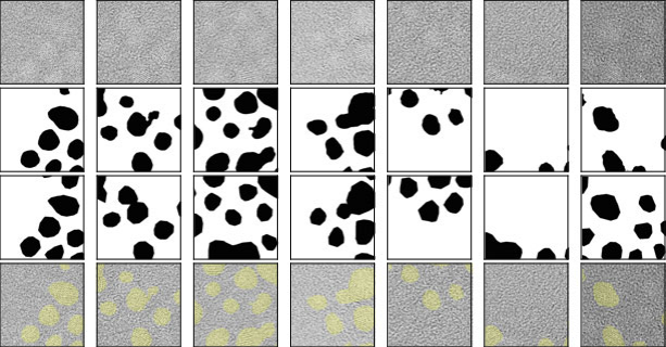
38. Voronoi tessellations for grain microstructures

The recipe. (Sandfeld et al. 2024) §19.3.2

1. Drop \(N\) random seed points in a 2D box.

2. Each pixel is assigned to the nearest seed (Voronoi cell).

3. The cell boundaries are exact grain boundaries.

4. Optionally: relax seed positions (Lloyd’s algorithm) for more regular grains.

Knobs.

• Number of seeds \(N\) \(\to\) grain size distribution.

• Seed-placement model (random / blue-noise / clustered) \(\to\) texture.

• Boundary thickness, smoothing \(\to\) visual realism.

• Anisotropy weights \(\to\) elongated grains (rolled metals).

• Generate millions of unique microstructures in seconds; perfect masks for free.

Synthetic polycrystalline microstructure generated by Voronoi tessellation, with the corresponding ground-truth grain-boundary mask.

Why Voronoi works as a model. Real polycrystalline metals form via nucleation-and-growth: grains nucleate at random sites and grow until they meet. The resulting microstructure is literally a Voronoi tessellation in the limit of equal growth rates. So the geometric model is physically motivated, not arbitrary.

Where Voronoi fails as a model.

• Grain growth: real grains grow at different rates depending on orientation, temperature, etc. Real grain-size distributions follow log-normal, not the more uniform distribution Voronoi produces.
• Recrystallization: introduces sub-grain structures Voronoi doesn’t capture.
• Rolling/drawing: introduces strong anisotropy.

For these, more sophisticated generators (phase-field, Monte Carlo Potts) are needed.

Implementation tips.

• scipy.spatial.Voronoi gives polygons; rasterize with cv2.fillPoly.
• For realistic boundary widths (typically 1–3 pixels), apply morphological dilation to the boundary mask.
• For variability, jitter the seed count, the seed positions, the boundary width, and the boundary anti-aliasing.

Connection to Random Field models (Unit 4 callback). The Voronoi construction is a special case of the random tessellation family; random fields more broadly include Boolean models (random circles for porosity), Poisson-line models (fiber networks), etc. Each captures a specific physics.

Bridge. Slide 39: turning the synthetic geometry into a synthetic image.

39. From geometry to image — the synthetic ladder

Step 1: clean geometry. Voronoi mask, binary boundaries.

Step 2: add texture. Per-grain intensity (random or orientation-dependent).

Step 3: add PSF blur. Gaussian blur with realistic \(\sigma_\text{psf}\).

Step 4: add noise. Poisson + Gaussian per detector model.

Step 5: add artifacts. Scan distortions, charging, gradients.

Each step closes a piece of the sim-to-real gap.

• Step 1 alone \(\to\) network learns to detect “perfect line on uniform background”; fails completely on real SEM.

• Through step 4 \(\to\) network learns to detect “blurred edges in noisy textured field”; works on most real SEM.

• Step 5 (artifact simulation) \(\to\) robustness to specific instrument quirks.

The “match the deployment distribution” principle. Each step in the ladder approximates a piece of the real-image generation process (Unit 2 material). The right amount of synthesis depends on the deployment distribution:

• For high-quality, low-noise images: steps 1–3 may suffice.
• For low-dose, noisy SEMs: steps 1–4 essential.
• For old microscopes with known artifacts: step 5 helps.

Practical recipe. I recommend starting with all five steps with mild parameters (matching the cleanest real images you have), then incrementally make the synthesis more aggressive (matching noisier real images). Validate at each level on real held-out data.

Connection to physics-based simulation. Steps 3–5 can be replaced by physical simulation — multi-slice for TEM, electron-beam Monte Carlo for SEM, finite-element for AFM. More accurate but much slower. Use physical simulation when the application demands it (e.g., quantitative intensity analysis); use the cheap “noise + blur” model when only geometric features matter.

An underappreciated trick: domain randomization. Instead of trying to exactly simulate the deployment distribution, randomize aggressively across many possible distributions. The network learns to be robust to any of them. This is the dominant approach in robotics sim-to-real and works well for materials too.

Bridge. Slide 40 makes the sim-to-real gap precise.

40. The Sim-to-Real gap

The phenomenon.

• Network trained on synthetic alone: 95 % validation IoU on synthetic.
• Same network on real images: 30–50 % IoU.
• The network learned features that are only present in synthetic.

Why it happens (optimization view).

• The synthetic loss surface \(\mathcal{L}_\text{syn}\) has minima at feature configurations that detect synthetic-specific artifacts.
• The real loss surface \(\mathcal{L}_\text{real}\) has minima elsewhere.
• A model perfectly fit to \(\mathcal{L}_\text{syn}\) is not even close to a minimum of \(\mathcal{L}_\text{real}\).

Closing the gap is two ML problems — better simulation, or domain adaptation (next slide).

The shortcut-learning failure mode. Networks find the easiest features that solve the training task. On synthetic data, the easiest feature is often a synthesis artifact: a perfectly straight boundary, an exact pixel-aligned color step, a noise-free background. Real images don’t have those features, so the model has nothing to attend to.

Diagnostic for sim-to-real failure.

• Generate adversarial-easy synthetic images (very clean, very simple); check the model is fitting them perfectly.
• Generate adversarial-hard synthetic images (more noise, more blur); check the model still works.
• Test on real images.
• If real \(\ll\) adversarial-hard, your synthetic distribution is too narrow — diversify.

The two strategies (next slides).

1. Better simulation (slide 39): make synthetic look more like real.
2. Domain adaptation (slide 41): train so the model is invariant to the difference.

The two are complementary; combine them.

Honest assessment. Sim-to-real is the unsolved problem of synthetic training. There is no magic bullet. Best practice is: aggressive synthetic diversity + small real fine-tuning set + careful held-out real evaluation.

Bridge. Slide 41: domain adaptation.

41. Domain adaptation

Strategy A: Make synthetic look real.

• Style transfer from real images onto synthetic (CycleGAN).
• Diffusion models conditioned on synthetic masks.
• Caveat: the generator must not change the labels.

Strategy B: Domain randomization.

• Vary synthesis parameters (noise, blur, contrast) aggressively.
• The model is forced to learn distribution-invariant features.
• Simpler than GANs; often equally effective.

Strategy C: Fine-tune on real.

• Pretrain on synthetic, fine-tune on a small real labeled set.
• Combines synthetic pretraining (rich feature learning) with real fine-tuning (closes the sim-to-real gap).
• Apply the full §2 fine-tuning recipe.

The pragmatic recommendation: Combine B (random synthesis) + C (real fine-tuning). Skip A unless you have GAN expertise.

Strategy A: synthetic→real style transfer. A GAN learns to take a synthetic image and “make it look real” without changing the microstructure. The generator is trained adversarially against a discriminator that distinguishes real from generated-real. Three practical issues:

1. Cycle consistency. CycleGAN-style models can sometimes change labels (a grain boundary moves when the texture is restyled). Mitigation: use a content-preserving variant (StarGAN, MUNIT) or add a label-consistency loss.
2. Training stability. GAN training is notoriously unstable. Modern diffusion-based variants are more reliable.
3. Compute. Training a CycleGAN is itself a research project.

Strategy B: domain randomization (Tobin et al. 2017). Born in robotics: instead of one fixed simulator, randomize the simulator across a wide range of parameters. The network learns to be invariant to the variation. For materials: randomize noise level, PSF width, contrast, brightness, scan distortion magnitude — all together — at training time. Empirically this is the easiest strategy that often works.

Strategy C: synthetic-pretrain + real-finetune. The §2 recipe applied to a synthetic-pretrained backbone:

1. Pretrain on synthetic with full §3 augmentation.
2. Replace head if necessary.
3. Apply the full §2 fine-tuning recipe on the small real dataset (discriminative LRs, warm-up, cosine, etc.).

This is the modern default. Even 10 real labeled images can dramatically close the sim-to-real gap.

Cascade pretraining (best of all worlds). ImageNet → synthetic materials → real materials. Three TL stages, each providing more specific features. This is the gold-standard pipeline.

Bridge. Slide 42 walks through a complete success case.

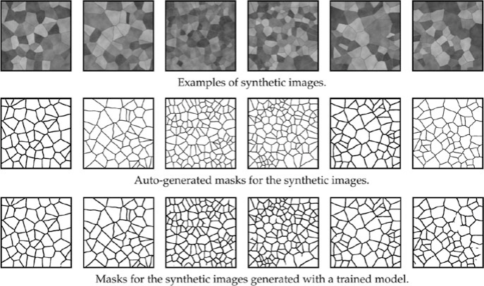
42. Case study — SEM grain segmentation on Voronoi

Setup. (Sandfeld et al. 2024) Fig 19.11

• Training. Voronoi-synthetic grain images + perfect masks. Augmentation: noise, blur, intensity jitter.
• Architecture. U-Net (ImageNet-pretrained encoder + scratch decoder).
• Deployment. Real polycrystalline SEM images (never seen in training).
• Goal. Predict grain-boundary masks on real data.

Outcome.

• Network trained only on synthetic generalizes to real SEMs.
• Captures the topology of grain networks (closed cells, triple junctions, no dangling boundaries).
• Far more accurate than classical edge detection (Canny, watershed), which is fooled by texture and noise.

Take-home. With careful augmentation, the synthetic→real transfer is real. No real labels were used.

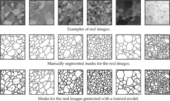
Real SEM image (left) and predicted grain-boundary mask (right) from a U-Net trained only on Voronoi synthetic data. The model captures the closed-cell topology characteristic of polycrystalline metals.

What’s actually being demonstrated. The model has never seen a real SEM image during training. Yet the predictions on real SEM are qualitatively correct — closed cells, triple junctions at ~120°, boundary-thickness consistency. That’s because the topological and geometric features of grain networks are captured by the Voronoi generator, and the augmentation hides the synthetic-specific noise characteristics.

Why classical methods fail here. Canny edge detection, watershed, and morphological operators all rely on pixel-intensity gradients. Real SEMs have intra-grain texture (orientation contrast, roughness) that also produces gradients — classical methods see those textures as “edges” and produce noisy, fragmented boundary predictions. The U-Net learned the topology of valid grain networks, so it suppresses texture-induced false edges.

Quantitative numbers (from Sandfeld). Classical Canny+watershed gives ~50–60 % IoU; the U-Net trained on Voronoi gives ~85–90 %.

The recipe components.

• ImageNet-pretrained encoder (slide 27): provides edge/texture features.
• Voronoi-synthetic data (slide 38): provides topology + perfect labels.
• Aggressive augmentation (§3): closes sim-to-real gap.
• U-Net architecture: well-suited to dense pixel-level prediction.

The honest caveat. Synthetic-only training works well enough but fine-tuning on even 5–10 real labeled SEMs typically closes the remaining gap. The §6 recipe is what you would do in production.

Foreshadowing W11/W14. Active learning would let us pick which 5 real images to label to maximize the gain — preview slide later.

43. Procedural generation beyond grains

Other domains where synthetic data shines.

• Spectra (XRD, EELS, EDXS): simulate peak positions, widths, Lorentzian/Voigt shapes, backgrounds. Train denoising and peak- identification networks.
• Diffraction patterns (4D-STEM): simulate Bragg disks for known crystal orientations. Train orientation-mapping networks.

• 3D microstructures: phase-field or Monte Carlo Potts simulations. Train 3D-segmentation networks.
• Defect statistics: generate dislocations, precipitates with controlled densities. Train defect-classification networks.

Across all of these, the recipe is the same:

1. Simulator generates labeled examples.
2. Augment to close sim-to-real gap.
3. Fine-tune on a small real labeled set.

Spectroscopy: the easiest case for synthetic data. Spectra are 1D, the physics is well-understood (peak shapes, broadening mechanisms, backgrounds), and the generation is fast. A network trained on simulated XRD spectra with realistic noise + background can identify phases in real diffractograms with high accuracy.

Materials groups around the world have published synthetic-trained networks for:

• XRD phase identification (e.g., (Park et al. 2017)).
• EELS edge identification.
• 4D-STEM orientation mapping (the “py4DSTEM” community).
• Atom finding in HRTEM (e.g., (Madsen et al. 2018)).
• Dislocation identification in TEM diffraction (e.g., the work of Sandfeld’s own group).

The Pelz-group connection. Several recent ptychographic-tomography papers from our group (Romanov et al. 2024; You et al. 2024) use simulation-based training for forward/inverse model networks. The “simulator” here is the multi-slice diffraction physics; “real” data comes from experimental 4D-STEM acquisitions (Pelz et al. 2023).

Bridge to §6. Synthetic data is the third lever and combines with TL (§4) and augmentation (§3) into the full materials-ML recipe of §6.

44. Synthetic-data summary

Take-homes.

• Synthetic data closes the labeling gap but opens a sim-to-real gap.

• Both gaps must be addressed: aggressive augmentation + (ideally) small real fine-tuning set.

• Domain randomization (vary synthesis parameters widely) is the cheapest, most effective sim-to-real tool.

• Cascade pretraining (ImageNet \(\to\) synthetic \(\to\) real) is the state-of-the-art workflow.

Optimization view (§2 callback).

• Synthetic pretraining lands you in a basin closer to the materials target than ImageNet alone.
• Real fine-tuning is then a small final adjustment.
• The same MFML W6 recipe applies at each stage:
  • Per-layer LRs, warm-up, cosine, Adam→SGD switch.
• Synthetic data is just another pretraining source.

The unifying view. Synthetic data is not a new technique — it is just another pretraining source. The optimization machinery of §2 is unchanged: each successive pretraining gives you a warmer start for the next stage.

The full pipeline (the recipe to memorize).

1. ImageNet-pretrained backbone (§4).
2. Synthetic-data pretraining (§5) with §3 augmentation.
3. Real-data fine-tuning (§4) with §2 discriminative LRs and schedules.
4. §6 validation hygiene (next section).

This is the pipeline. Variations on it are the materials-ML literature.

When not to bother with synthetic data.

• If you have \(\geq 1000\) real labeled images, synthetic adds little.
• If your simulator is unfaithful to real physics in important ways, synthetic hurts.
• If your domain has no good simulator (rare phenomena, novel sample systems), synthetic isn’t an option.

When synthetic data is essential.

• Truly tiny datasets (\(< 50\) real labels).
• Tasks where labeling is fundamentally hard (3D microstructures, rare defects).
• Tasks where simulation is well-trusted (Voronoi for grains, Bragg for diffraction).

Bridge. §6 brings everything together into the practical recipe.

§6 · Practical Workflow & Best Practices

Section purpose. §6 is the deliverable: the explicit workflow students should follow next time they have a small materials dataset and a fine-tuning task. The recipe synthesizes §2 (optimization), §3 (augmentation), §4 (transfer learning), and §5 (synthetic data) into a single, actionable checklist.

Validation hygiene is the second half — without it, all of the above is vulnerable to silent failure modes (data leakage, augmentation contamination, group leakage). Unit 3’s K-fold material is the foundation we build on here.

45. The fine-tuning recipe — the canonical workflow

Steps.

1. Pick a pretrained backbone (ResNet-50 / ConvNeXt / ViT-B).

2. Replace the head for your number of classes / output channels.

3. Freeze backbone; train head with Adam, LR \(\sim 10^{-3}\).

4. Unfreeze with discriminative LRs + warm-up + cosine schedule.

5. Switch to SGD+momentum for the last \(\sim 20\%\) of steps.

6. Augment throughout (geometric + intensity + noise).

7. Validate with grouped K-fold; held-out test on a different sample.

Map back to MFML W6.

Step	MFML W6 idea
1, 3	Warm start in flat basin
4	Per-parameter LR + schedule + warm-up
5	Adam → SGD+momentum (flat minima)
6	Effective dataset size + invariances
7	Generalization measurement

• Every step of this recipe is a direct application of MFML W6.
• The recipe is the deliverable of this unit.

The canonical materials-ML workflow. This is the recipe I would hand to a new graduate student starting their first ML project. Every piece is justified by §§2–5; no piece is optional for small materials datasets.

One-page implementation plan to write on the board.

Day 1: Set up dataset; define grouped K-fold splits.
Day 2: Train scratch baseline (sanity check).
Day 3: Feature extraction with ImageNet-pretrained backbone.
Day 4: Add augmentation (geometric + intensity).
Day 5: Full fine-tuning with discriminative LRs, warm-up, cosine.
Day 6: Add SGD-momentum final phase.
Day 7: Add synthetic-data pretraining (if applicable).
Day 8: Held-out test on different sample / microscope.

Stopping criteria at each stage. Each stage should measurably improve held-out performance. If a stage doesn’t help, debug it before moving on. Common debugging:

• Augmentation hurts: too aggressive, or violating physical legality.
• TL hurts: catastrophic forgetting (LR too large) or wrong source domain.
• Synthetic hurts: sim-to-real gap, simulator bug.

The mindset shift to convey. Materials ML is not “pick an architecture and tune hyperparameters.” It is “stack pretraining stages and validate at each step.” The recipe makes this explicit.

Bridge. Slides 44–45 cover the validation half.

46. Validation in the small-data regime

The problem. With \(N=100\) images:

• A single 80/20 train/test split gives \(\sim 20\) test images.
• Standard error on accuracy is \(\pm 5\)–\(10\) percentage points.
• One run is not enough to claim a result.

The solution: K-fold cross-validation (Unit 3 callback).

• Split data into \(K\) folds; train \(K\) models, each holding one fold.
• Average across folds; report mean ± stddev.
• Standard \(K = 5\); for very small data \(K\) up to \(N\) (LOOCV).

• Mandatory for any small-data result. A single train/val/test split is a publication risk.

Why K-fold matters in materials ML specifically. With \(N=100\) and 20 % test, your test set is ~20 images. The variance of test accuracy across random splits is enormous — different splits routinely give results 10+ points apart. Without K-fold, your “result” is a sample of size 1 from a high-variance distribution.

K-fold cost. Training \(K\) models takes \(K \times\) time. For modern materials-ML projects this is rarely the bottleneck (a \(K=5\) U-Net training fits in a day on a single GPU). Skipping K-fold to “save time” is false economy.

The reporting standard. When publishing or submitting work:

• Report mean ± stddev across folds.
• Report per-fold numbers in supplementary material.
• Use the same folds when comparing methods (a paired test).

Statistical tests. For comparing two methods, use a paired t-test across the K fold-pair differences. Don’t compare just the mean — small mean differences with overlapping intervals are not significant.

LOOCV (leave-one-out CV). For very small datasets (\(N < 30\)), \(K = N\). Computationally heavy but the only honest approach.

Bridge to slide 47. K-fold alone is not enough — which fold split matters. Group K-fold prevents augmentation/specimen leakage.

47. Group-based splitting — the leakage you don’t see

The trap.

• \(N=100\) images, but only \(5\) specimens.
• Random 80/20 split: each specimen contributes some images to train and some to test.
• The “test” measures within-specimen generalization, not cross- specimen generalization.
• Apparent test accuracy is vastly inflated.

The fix: group by specimen.

• 5 specimens, 5-fold CV: each specimen is the test in exactly one fold.
• Each fold trains on 4 specimens, tests on 1.
• Measures real cross-specimen generalization.

The bigger principle.

Whatever varies in deployment, must vary across train/test in your validation.

• Specimen, microscope, operator, day, batch — split the relevant axis.

The single most common silent failure in materials ML. Random splitting on a dataset where multiple images come from the same specimen (or operator, or day) systematically inflates accuracy. The model memorizes specimen-specific features (texture, drift pattern, residual contamination) and exploits them at test time because the same specimen is in both sets.

The diagnostic question. Before any validation, ask: what is the unit of generalization in my deployment scenario?

• If deploying on new specimens of the same alloy: split by specimen.
• If deploying on new alloys: split by alloy.
• If deploying on a new microscope: split by microscope.
• If deploying across multiple labs: split by lab.

If you do not have enough distinct units to support a K-fold split on the right axis, you do not have enough data to claim cross-axis generalization — period. Collect more, or restrict your claim.

Augmentation-induced leakage (§3 callback, slide 25). A special case: if the same image and its rotation end up on both sides of the split, the test is easy in a way that has nothing to do with materials science. Always split before augmenting.

Implementation. sklearn.model_selection.GroupKFold takes a groups array (one entry per sample identifying its group). Use it.

The reviewer-pleasing standard. Report results with two split strategies:

1. Random K-fold (the optimistic estimate).
2. Group K-fold by specimen (the honest estimate).

The gap between them tells the reader how much specimen-specific overfitting your model is doing. Honest reporting builds trust.

Bridge. Slide 48: active learning — the next-level optimization of which labels to acquire.

48. Active learning — bonus concept

The idea.

• You can label some images, but not all.
• Which images should you label?
• Active learning: label the images where the current model is least confident.

Why this works.

• Confident predictions teach the model little (already correct).
• Uncertain predictions are at the decision boundary — labeling them carries the most information.
• Maximizes the value per expert-hour.

Foreshadowing. Full treatment in W11 (automation) and W14 (Bayesian experiment design). Today: just know it exists and is the smart way to allocate your labeling budget.

The active-learning loop.

1. Train initial model on a small seed labeled set.
2. Run inference on the unlabeled pool.
3. Score each unlabeled image by uncertainty (e.g., predictive entropy).
4. Label the top-K most uncertain images.
5. Add to training set; retrain.
6. Repeat until budget exhausted.

Uncertainty quantification. “Confidence” = high softmax probability is a bad proxy in deep nets (Guo et al. 2017). Better proxies:

• Predictive entropy of the softmax output.
• MC-dropout ensemble: sample multiple forward passes with dropout active; measure prediction variance.
• Deep ensembles: train \(M\) networks, take variance.
• Bayesian deep learning (W12 / GP material).

Empirical impact. On materials problems, active learning typically matches passive (random) labeling at 2–5× fewer labels. For high-cost labels (materials science!), this is enormous.

The paradox. Active learning requires a working initial model — so you still need a baseline labeled set. The combination “small seed + active loop + transfer learning” is the modern small-data workflow.

Forward links.

• W11: automation, where active learning is closed-loop with the microscope.
• W12: GP-based active learning for regression problems.
• W14: integration with Bayesian experiment design.

Bridge. Slide 49: the gold-standard test set.

49. The gold-standard test set

The principle.

A small, never-augmented, never-touched test set is non-negotiable.

• Reserve \(10\)–\(20\) examples on a different specimen / microscope / day.
• Lock them away. Touch them only at the end.
• Never use them for hyperparameter tuning.

Why this matters.

• The K-fold validation tells you about one slice of the distribution.

• The gold-standard test is your external check.

• Iterating on the validation set \(\Rightarrow\) overfit the validation set.

• The gold-standard test catches that overfitting.

• If you check the gold-standard test more than once, it stops being a gold-standard test.

The validation-set-overfitting failure mode. With small datasets, your validation set is small (\(\sim 20\) images). Over the course of a project, you might evaluate 100s of model variants on it. Each evaluation gives you a small amount of information about which variant is best — but you are implicitly fitting the validation set with your model selection. The “best” model on validation will overestimate true performance.

This is meta-overfitting and it is real. The only protection is a held-out test set you check exactly once.

The “exactly once” rule. If you check the gold-standard test set during development, you have leaked information from it into your modeling decisions. The set is now no longer gold-standard. New rules: establish the gold-standard test up front, don’t touch it until the paper is being written, report the result that comes out, accept it.

A practical compromise: held-out sets at multiple scales.

• Validation (used many times): used for hyperparameter search, model selection.
• Test (used a few times): used at the end of major phases.
• Gold-standard (used once): the final number for the paper.

The numbers should be in increasing order: gold-standard < test < val. If they are equal, you didn’t iterate enough; if gold-standard is dramatically lower, you overfit the validation.

Specific recommendation. For an honest small-data result: 80 % train + augment, 10 % validation (multiple uses), 10 % gold-standard (used once). Stratified by group/specimen.

Bridge. Slide 50 covers when to stop training.

50. When to stop — early stopping

The mechanic.

• Track validation loss every epoch.
• If validation loss has not improved for \(P\) epochs (patience), stop.
• Restore the best validation checkpoint.

# PyTorch Lightning
EarlyStopping(monitor="val_loss",
              patience=10,
              mode="min")

Why early stopping is essential for fine-tuning.

• Small datasets are prone to late-stage overfitting: validation loss starts climbing while train loss keeps falling.
• Without early stopping, the final epoch’s checkpoint is overfit and worse than an earlier one.

Combine with cosine schedule. Cosine reduces LR toward zero, so by the end of training, gradient steps are small and overfitting is gentle. But early stopping is still cheap insurance.

Early stopping as implicit regularization. From the optimization perspective (MFML W6), early stopping is equivalent to L2 regularization for linear models — both shrink the solution toward the initialization. For non-linear deep networks, the equivalence is approximate but the intuition holds: stopping early keeps you near your starting point, which for fine-tuning is the pretrained point — exactly the basin we want to stay in.

Patience selection.

• Typical patience: \(P = 10\) for fine-tuning, \(P = 20\) for from-scratch training.
• For very small datasets, \(P\) may need to be \(> 20\) — validation loss is noisy on small validation sets, so don’t stop on first noise spike.

The “best checkpoint” trap. A common bug: training script stops on patience, but doesn’t restore the best checkpoint, only the latest. The latest is the worst of the recent ones. Always restore the best-validation checkpoint.

Combining early stopping with K-fold. Each fold’s training has its own early stopping; report the average best-epoch performance, not the fixed-epoch performance.

Caveat. With cosine annealing to (near-)zero LR, the model often converges cleanly without overfitting late in training. In that case early stopping rarely fires, and the cosine schedule alone provides the stopping behavior. Still set early-stopping as a safety net.

Forward link. W14 covers the relationship between early stopping, implicit bias, and generalization in deeper detail.

51. Top takeaways

1. Fine-tuning is continued optimization. Every MFML W6 lesson applies — flat basins, per-layer LRs, schedules, batch noise.

2. Augment to encode physical invariances. Don’t break physics. Don’t leak.

3. Transfer from large-scale pretraining (ImageNet) and / or synthetic data. Cascade is best.

4. Synthetic data closes the labeling gap; aggressive augmentation closes the sim-to-real gap.

5. Validate with grouped K-fold + a true gold-standard test on a different specimen / microscope.

6. The recipe is the deliverable: backbone choice → head replace → freeze/unfreeze with discriminative LRs → warm-up + cosine → Adam→SGD switch → augment → group K-fold.

7. Modern levers when ImageNet is not enough: self-supervised backbones (DINOv2, MAE-on-lab-data) for features, and memory-light optimizers (Lion) for fitting larger models on lab GPUs.

The take-home in one sentence. Never train from scratch when somebody — ImageNet, a synthetic generator, a previous lab — has already paid the optimization bill for you; and validate ruthlessly with grouped K-fold against a gold-standard test set.

Connecting back to MFML W6. Six points; five of them are direct applications of optimization theory:

• 1. is the optimization framing itself.
• 2. is loss-surface smoothing via averaged inputs.
• 3. is warm-start initialization.
• 4. is cascaded warm-start initialization.
• 6. is the synthesis of MFML W6 mechanics.

Only (5) is “purely” statistical hygiene. Even there, the why of K-fold (variance reduction) is an optimization-theoretic argument about estimator variance with small samples.

The pedagogical arc. Unit 6 took you from “small data is hard” to “optimization theory tells us exactly what to do about it.” Every practical recipe — discriminative LRs, gradual unfreezing, synthetic pretraining, group K-fold — drops out of the §2 framing.

For the rest of the course.

• W7 (time series): the same recipe, with temporal augmentations.
• W8 (generalization, robustness): how the recipe holds across process windows.
• W11 (automation): closes the loop with active learning.
• W12 (Gaussian processes): an alternative path for very small data with uncertainty.
• W13 (PINNs): physics-as-prior, the next level of “physics-informed” augmentation.
• W14 (reflection): integrates these into the materials-ML practice.

Bridge to references. Slide 52: where to read more.

52. References & further reading

Course textbooks.

• (Sandfeld et al. 2024), Ch. 19 — transfer learning, augmentation, synthetic data; Au-nanoparticle U-Net (§19.3.1) and Voronoi grain segmentation (§19.3.2).
• (McClarren 2021), Ch. 6 — CNNs and large datasets, with practical examples.
• (Neuer et al. 2024) — physics-informed and explainable methods for engineering.
• (Goodfellow et al. 2016) — Ch. 8 (Optimization for Training Deep Models) is the textbook reference for §2.

53. References & further reading 2

Foundational references. (Howard and Ruder 2018) ULMFiT — discriminative fine-tuning; (Loshchilov and Hutter 2017) SGDR — warm restarts and cosine annealing; (Smith 2017) — LR-finder; (Wilson et al. 2017) — marginal value of adaptive methods; (Goyal et al. 2017) — linear-scaling rule; (Tobin et al. 2017) — domain randomization; (Kumar et al. 2022) — fine-tuning vs. linear probing; (Yosinski et al. 2014) — how transferable are features in deep neural networks.

MFML cross-reference. Unit 6 of the MFML course (this same week) covers loss landscapes, SGD/Adam, learning-rate schedules, and the batch–noise trade-off. Every practical recipe in this lecture is a direct application of that material.

Closing remarks. The references are organized by role, not by chronological order. Read Sandfeld first (textbook), then Goodfellow Ch. 8 (theory), then the original papers (depth).

Pivotal TL papers cited in this lecture:

• (Howard and Ruder 2018), “Universal Language Model Fine-tuning for Text Classification” — the discriminative-fine-tuning paper.
• (Loshchilov and Hutter 2017), “SGDR: Stochastic Gradient Descent with Warm Restarts.”
• (Smith 2017), “Cyclical Learning Rates for Training Neural Networks” (LR-finder).
• (Wilson et al. 2017), “The Marginal Value of Adaptive Gradient Methods in Machine Learning.”
• (Yosinski et al. 2014), “How Transferable Are Features in Deep Neural Networks?”
• (Tobin et al. 2017), “Domain Randomization for Transferring Deep Neural Networks from Simulation to the Real World.”
• (Kumar et al. 2022), “Fine-tuning Can Distort Pretrained Features and Underperform Out-of-Distribution.”

If students want the historical arc of TL, those papers (plus (Donahue et al. 2014; Razavian et al. 2014)) are the reading list.

A final thought to leave them with. Materials ML is a cumulative discipline. Every successful project stands on top of the optimization work of the ImageNet community, the synthetic-data work of the microstructure-modeling community, and the validation-hygiene work of the statistics community. Recognize what others have done; reuse it ruthlessly; do your own work on top.

Next time (W7): from images to time series. The same optimization machinery, applied to process-monitoring signals.

Continue

• ← Previous: Unit 05 — Unsupervised methods for materials — clustering & autoencoders
• → Next: Unit 07 — Generalization, robustness, and process windows
• All courses

References

Chen, Ting, Simon Kornblith, Mohammad Norouzi, and Geoffrey Hinton. 2020. “A Simple Framework for Contrastive Learning of Visual Representations.” International Conference on Machine Learning (ICML). https://arxiv.org/abs/2002.05709.

Chen, Xiangning, Chen Liang, Da Huang, et al. 2023. “Symbolic Discovery of Optimization Algorithms.” Advances in Neural Information Processing Systems.

Donahue, Jeff, Yangqing Jia, Oriol Vinyals, et al. 2014. “DeCAF: A Deep Convolutional Activation Feature for Generic Visual Recognition.” International Conference on Machine Learning (ICML).

Goodfellow, Ian, Yoshua Bengio, and Aaron Courville. 2016. Deep Learning. MIT Press.

Goyal, Priya, Piotr Dollár, Ross Girshick, et al. 2017. “Accurate, Large Minibatch SGD: Training ImageNet in 1 Hour.” arXiv Preprint arXiv:1706.02677.

Guo, Chuan, Geoff Pleiss, Yu Sun, and Kilian Q. Weinberger. 2017. “On Calibration of Modern Neural Networks.” International Conference on Machine Learning, 1321–30.

He, Kaiming, Xinlei Chen, Saining Xie, Yanghao Li, Piotr Dollár, and Ross Girshick. 2022. “Masked Autoencoders Are Scalable Vision Learners.” Proceedings of the IEEE/CVF Conference on Computer Vision and Pattern Recognition (CVPR), 16000–16009.

Howard, Jeremy, and Sebastian Ruder. 2018. “Universal Language Model Fine-Tuning for Text Classification.” Proceedings of the 56th Annual Meeting of the Association for Computational Linguistics (Volume 1: Long Papers), 328–39.

Keskar, Nitish Shirish, Dheevatsa Mudigere, Jorge Nocedal, Mikhail Smelyanskiy, and Ping Tak Peter Tang. 2017. “On Large-Batch Training for Deep Learning: Generalization Gap and Sharp Minima.” International Conference on Learning Representations.

Kumar, Ananya, Aditi Raghunathan, Robbie Jones, Tengyu Ma, and Percy Liang. 2022. “Fine-Tuning Can Distort Pretrained Features and Underperform Out-of-Distribution.” International Conference on Learning Representations.

Li, Hao, Zheng Xu, Gavin Taylor, Christoph Studer, and Tom Goldstein. 2018. “Visualizing the Loss Landscape of Neural Nets.” Advances in Neural Information Processing Systems 31.

Liu, Yang, Yuda Li, Soojin Jeong, Yi Wang, Jun Chen, and Xingchen Ye. 2020. “Colloidal Synthesis of Nanohelices via Bilayer Lattice Misfit.” Journal of the American Chemical Society 142 (29): 12777–83. https://doi.org/10.1021/jacs.0c05175.

Loshchilov, Ilya, and Frank Hutter. 2017. “SGDR: Stochastic Gradient Descent with Warm Restarts.” International Conference on Learning Representations.

Madsen, Jacob, Pei Liu, Jens Kling, et al. 2018. “A Deep Learning Approach to Identify Local Structures in Atomic-Resolution Transmission Electron Microscopy Images.” Advanced Theory and Simulations 1 (8): 1800037. https://doi.org/10.1002/adts.201800037.

Mandt, Stephan, Matthew D. Hoffman, and David M. Blei. 2017. “Stochastic Gradient Descent as Approximate Bayesian Inference.” Journal of Machine Learning Research 18 (1): 4873–912.

McCandlish, Sam, Jared Kaplan, Dario Amodei, and OpenAI Dota Team. 2018. “An Empirical Model of Large-Batch Training.” arXiv Preprint arXiv:1812.06162.

McClarren, Ryan G. 2021. Machine Learning for Engineers: Using Data to Solve Problems for Physical Systems. Springer.

Neuer, Michael et al. 2024. Machine Learning for Engineers: Introduction to Physics-Informed, Explainable Learning Methods for AI in Engineering Applications. Springer Nature.

Neyshabur, Behnam, Hanie Sedghi, and Chiyuan Zhang. 2020. “What Is Being Transferred in Transfer Learning?” Advances in Neural Information Processing Systems 33: 512–23.

Oquab, Maxime, Timothée Darcet, Théo Moutakanni, et al. 2024. “DINOv2: Learning Robust Visual Features Without Supervision.” Transactions on Machine Learning Research.

Park, Woon Bae, Jiyong Chung, Jaeyoung Jung, et al. 2017. “Classification of Crystal Structure Using a Convolutional Neural Network.” IUCrJ 4 (4): 486–94. https://doi.org/10.1107/S205225251700714X.

Pelz, Philipp M., Sinéad M. Griffin, Scott Stonemeyer, et al. 2023. “Solving Complex Nanostructures with Ptychographic Atomic Electron Tomography.” Nature Communications 14 (11): 7906. https://doi.org/10.1038/s41467-023-43634-z.

Razavian, Ali Sharif, Hossein Azizpour, Josephine Sullivan, and Stefan Carlsson. 2014. “CNN Features Off-the-Shelf: An Astounding Baseline for Recognition.” Proceedings of the IEEE Conference on Computer Vision and Pattern Recognition Workshops, 806–13.

Romanov, Andrey, Min Gee Cho, Mary Cooper Scott, and Philipp Pelz. 2024. “Multi-Slice Electron Ptychographic Tomography for Three-Dimensional Phase-Contrast Microscopy Beyond the Depth of Focus Limits.” Journal of Physics: Materials 8 (1): 015005. https://doi.org/10.1088/2515-7639/ad9ad2.

Ronneberger, Olaf, Philipp Fischer, and Thomas Brox. 2015. “U-Net: Convolutional Networks for Biomedical Image Segmentation.” Medical Image Computing and Computer-Assisted Intervention (MICCAI). https://arxiv.org/abs/1505.04597.

Sandfeld, Stefan et al. 2024. Materials Data Science. Springer.

Smith, Leslie N. 2017. “Cyclical Learning Rates for Training Neural Networks.” 2017 IEEE Winter Conference on Applications of Computer Vision (WACV), 464–72.

Tobin, Josh, Rachel Fong, Alex Ray, Jonas Schneider, Wojciech Zaremba, and Pieter Abbeel. 2017. “Domain Randomization for Transferring Deep Neural Networks from Simulation to the Real World.” 2017 IEEE/RSJ International Conference on Intelligent Robots and Systems (IROS), 23–30.

Wilson, Ashia C., Rebecca Roelofs, Mitchell Stern, Nati Srebro, and Benjamin Recht. 2017. “The Marginal Value of Adaptive Gradient Methods in Machine Learning.” Advances in Neural Information Processing Systems 30.

Yosinski, Jason, Jeff Clune, Yoshua Bengio, and Hod Lipson. 2014. “How Transferable Are Features in Deep Neural Networks?” Advances in Neural Information Processing Systems 27.

You, Shengbo, Andrey Romanov, and Philipp M Pelz. 2024. “Near-Isotropic Sub-Ångstrom 3d Resolution Phase Contrast Imaging Achieved by End-to-End Ptychographic Electron Tomography.” Physica Scripta 100 (1): 015404. https://doi.org/10.1088/1402-4896/ad9a1a.