Machine Learning in Materials Processing & Characterization
Unit 6: Data Scarcity & Transfer Learning


07. The “Small Data” Survival Kit
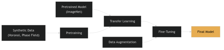
Three strategies to overcome data scarcity:
- Data Augmentation: Multiply data by applying valid transformations
- Transfer Learning: Reuse knowledge from large-dataset models
- Synthetic Training: Generate labeled data for free using simulations
18. The Label Consistency Rule
If you transform the image, you must transform the labels identically!
- Rotate image → rotate mask
- Flip image → flip mask
- Crop image → crop mask at the same location
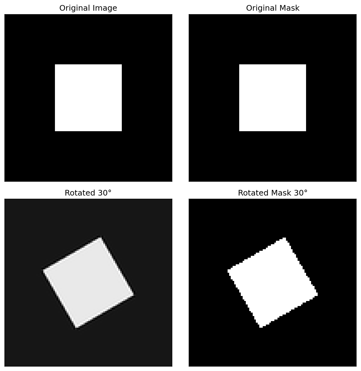
Intensity augmentations (brightness, noise) don’t affect labels — only geometric ones do.
23. The Backbone and the Head
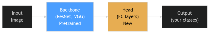
- Backbone: The feature extractor — pretrained on ImageNet
- Head: The classifier/regressor — newly initialized for your task
- Replace the head to match your number of classes
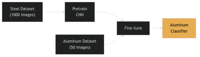
29. Cross-Material Transfer
- Train on a large database of steel micrographs
- Fine-tune on a small set of aluminum samples
- Physics intuition: Grain boundary topology is similar across alloy systems
30. Success Story: Au Nanoparticle Segmentation
- Task: Segment crystalline Au nanoparticles from amorphous TEM background
- Method: U-Net initialized with ImageNet weights
- Result: High accuracy despite limited labeled TEM frames
ImageNet pretraining helped even though ImageNet contains no TEM images — the low-level features transferred.
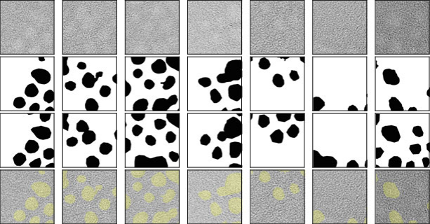
33. The “Infinite Data” Dream
- Simulate the structure → generate unlimited labeled data
- Perfect masks for free — no expert annotation
- Controllable — sweep grain size, defects, dose, aberrations at will
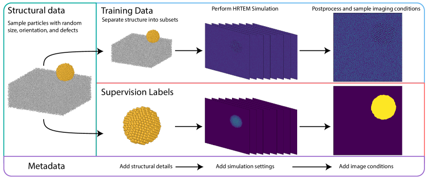
Note
The labeling arrow flips: instead of labeling real images, we render images from known structures.
Made concrete — Construction Zone (Rakowski et al., npj Comput. Mater. 10, 165, 2024): build thousands of random Au nanoparticles on carbon → multislice HRTEM simulation → physical post-processing (thermal, aberrations, plasmon loss, Poisson noise) → segmentation masks by construction.
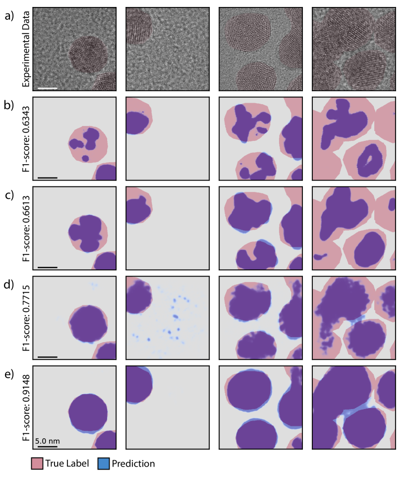
34. …And It Works: Purely Synthetic Beats Experimental SOTA
A U-Net trained only on simulated HRTEM — zero experimental images in training — segmenting real Au / CdSe nanoparticles:
| Benchmark | Synthetic-trained F1 | Prev. best (real-trained) |
|---|---|---|
| Au, large (5 nm) | 0.92 | 0.89 |
| Au, small (2.2 nm) | 0.86 | 0.75 |
| CdSe (2 nm) | 0.75 | 0.59 |
Important
The twist: what mattered was imaging-condition diversity + simulation fidelity — not the number of unique atomic structures. Simulate the right variation, not more structures.
35. Generating Grain Microstructures
Voronoi Tessellations:
- Distribute random seed points in 2D
- Assign each pixel to its nearest seed → grain regions
- Parameters: number of seeds (grain count), regularity, boundary thickness
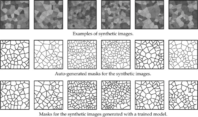
36. From Geometry to Realistic Image
A raw Voronoi diagram doesn’t look like an SEM image. We need to add:
- Grain contrast: Random intensity per grain
- Boundary appearance: Thickened, possibly bright or dark boundaries
- Texture: Per-grain crystallographic texture
- Noise: Gaussian + Poisson to simulate detector noise
- Blur: Slight defocus
39. Case Study: SEM Grain Segmentation
- Model trained only on Voronoi synthetic data
- Tested on real polycrystalline SEM images
- Result: Nearly perfect grain boundary segmentation!
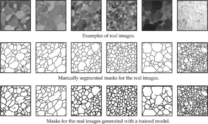
The synthetic data captured the topological truth of grain networks — boundaries, junctions, and connectivity patterns.
46. Group-Based Splitting Revisited
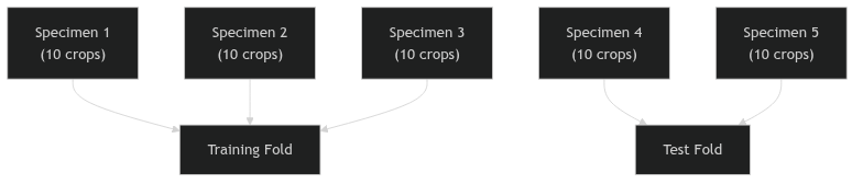
- If you have 5 specimens with 10 crops each = 50 images
- Split by specimen: 3 train, 2 test (not 40 random/10 random!)
- Then augment the 30 training images to 300+